Loops & Iteration
Learning Objectives:
- Manipulate Vectors and Lists using Base R syntax.
- Apply techniques of iteration to reduce and simplify your code.
Vectors
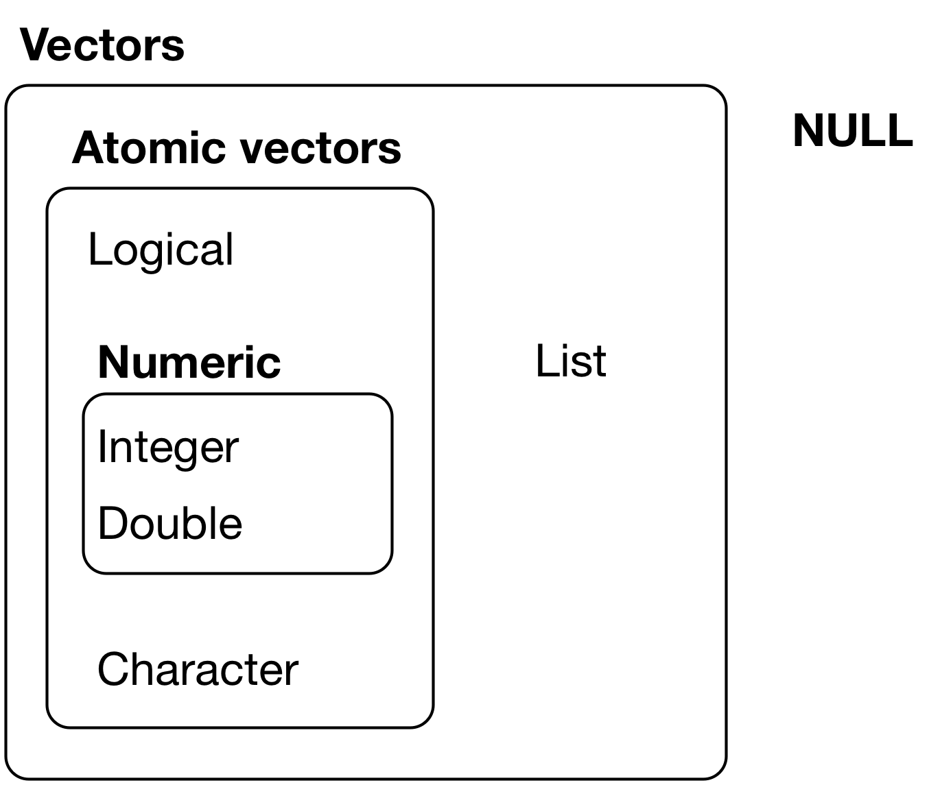
R has Only Two Kinds of Vectors: Atomic Vectors and Lists
- Atomic vectors are sequences of elements of the same data type.
- Lists are data structures where the elements do Not have to be the same type
- Sometimes called recursive vectors because lists can contain other lists!
- Vectors have two main attributes: Length and data Type
R has Six Data Types
The six data types are:
1. logical,
2. integer,
3. double,
4. character,
5. complex, and
6. raw(byte-level data).
factor, or date are special encodings of data types integer and double.
Integer and double vectors are collectively known as numeric vectors. Missing
Vectors return NULL, like missing or empty values in a vector can return NA.
Creating Vectors
- Use
c()to create a vector from the argument elements. - use
length()to see the length of a vector - Use
typeof()to see the type of vector - Use
is_*()to check the type of vector (from packagepurrr)- e.g.,
is_numeric(),is_logical,is_character, … - base R has similar functions
is.*()
- e.g.,
library(tidyverse)
## -- Attaching packages --------------------------------------- tidyverse 1.3.0 --
## v ggplot2 3.3.3     v purrr   0.3.4
## v tibble  3.1.0     v dplyr   1.0.3
## v tidyr   1.1.2     v stringr 1.4.0
## v readr   1.4.0     v forcats 0.5.1
## -- Conflicts ------------------------------------------ tidyverse_conflicts() --
## x dplyr::filter() masks stats::filter()
## x dplyr::lag()    masks stats::lag()
# - Double:
double <- c(1, 10, 2)
length(double)
## [1] 3
typeof(double)
## [1] "double"
is_double(double) ## From purrr package
## [1] TRUE
# - Integer: use `L` to tell R to treat (store) a number as an integer:
int <- c(1L, 10L, 2L)
typeof(int)
## [1] "integer"
is_integer(int) ## From purrr package
## [1] TRUE
# - Character:
char <- c("hello", "good", "sir")
length(char)
## [1] 3
typeof(char)
## [1] "character"
is_character(char) ## From purrr package
## [1] TRUE
# - Logical:
logi <- c(TRUE, FALSE, FALSE)
typeof(logi)
## [1] "logical"
is_logical(logi) ## From purrr package
## [1] TRUE
# - Factor: Factors are actually integers with extra attributes.
fac <- factor(c("A", "B", "B"))
fac
## [1] A B B
## Levels: A B
typeof(fac)
## [1] "integer"
is.factor(fac)
## [1] TRUE
class(fac)
## [1] "factor"
levels(fac) # to get the level labels
## [1] "A" "B"
as.numeric(fac) # to get the integers```
## [1] 1 2 2
# - Dates: Dates are actually doubles with extra attributes.
#   + Dates are the number of days since January 1, 1970, with negative values for earlier date
#   + The POSIXct class stores date/time values as the *number of seconds* since January 1, 1970

dat <- lubridate::ymd(20150115, 20110630, 20130422)
dat
## [1] "2015-01-15" "2011-06-30" "2013-04-22"
length(dat)
## [1] 3
typeof(dat)
## [1] "double"
class(dat)
## [1] "Date"
lubridate::is.Date(dat)
## [1] TRUE
purrr::is_double(dat) ## From purrr package
## [1] TRUE
Working with Elements in a Vector
Each element of a vector can have a name
x <- c(horse = 7, man = 1, dog = 8)
x
## horse   man   dog
##     7     1     8
Subset with brackets [...]
- Brackets are an extract or replace operator (see help for
extract()) - The index object
...can be numeric, logical, character or empty. - Putting a logical vector inside the brackets returns (extracts) the elements from the outer vector where the corresponding value in the inner logical vector is
TRUE
x <- c("I", "like", "dogs")
x[2:3]
## [1] "like" "dogs"
lvec <- c(TRUE, FALSE, TRUE)
x[lvec]
## [1] "I" "dogs"
See and set/change element names with the names() function
names(x)
## NULL
names(x)[1] <- "cat" #1 is the first element
x
##    cat   <NA>   <NA>
##    "I" "like" "dogs"
Extract with negative values to drop elements
x[-3]
##    cat   <NA>
##    "I" "like"
Extract a named vector with the name(s) of the desired element(s) as a character vector
x <- c(horse = 7, man = 1, dog = 8)
x[c("man", "horse")]
##   man horse
##     1     7
- Two brackets
[[...]]only extracts a single element and drops the name.
- The
[[...]]operator performs the[...]operation twice - Reduces an atomic vector to a named element and then extracts the element out of the named element
- Useful in working with lists (later on)
x[3]
## dog
##   8
x[[3]]
## [1] 8
Lists
Creating Lists
Lists are vectors whose elements can be of different types. A tibble or data
frame is a special kind of list (organized by columns with the same element
types in them). Use list() to make a list. It has a length: the number of
elements in the list. Each element in a list can have many elements in it. The
length of the list is just how many elements are present at the top level of the
list.
my_first_list <- list(x = "a", y = 1, z = c(1L, 2L, 3L), list("a", 1))
my_first_list
## $x
## [1] "a"
##
## $y
## [1] 1
##
## $z
## [1] 1 2 3
##
## [[4]]
## [[4]][[1]]
## [1] "a"
##
## [[4]][[2]]
## [1] 1
length(my_first_list)
## [1] 4
The above list, of length 4, has three named elements:
- a character
a - a numeric
1 - a logical vector
c(1L, 2L, 3L) - then it has an un-named list as the fourth element.
- The internal unnamed list has two elements
("a", 1)also unnamed.
- The internal unnamed list has two elements
- Use
str()(for structure) to see the internal properties of a list.
str(my_first_list)
## List of 4
##  $ x: chr "a"
##  $ y: num 1
##  $ z: int [1:3] 1 2 3
##  $  :List of 2
##   ..$ : chr "a"
##   ..$ : num 1
Working with Lists
- Single brackets
[...]extract a sublist. You use the same extracting strategies as for vectors.
my_first_list[1:2]
## $x
## [1] "a"
##
## $y
## [1] 1
str(my_first_list[1:2])
## List of 2
##  $ x: chr "a"
##  $ y: num 1
my_first_list["y"]
## $y
## [1] 1
my_first_list["z"]
## $z
## [1] 1 2 3
- Double brackets
[[...]]extract a single list element (which could also be a list).
- Each set of brackets subsets one layer
my_first_list[[1]]
## [1] "a"
my_first_list[["z"]]
## [1] 1 2 3
str(my_first_list[["z"]])
## int [1:3] 1 2 3
- Use dollar signs
$to extract named list elements (just like in data frames).
my_first_list$z
## [1] 1 2 3
Loops
In our last lesson on functions, we talked about how important it is to reduce duplication in your code by creating functions instead of copying-and-pasting. Reducing code duplication has three main benefits:
- It’s easier to see the intent of your code, because your eyes are drawn to what’s different, not what stays the same.
- It’s easier to respond to changes in requirements. As your needs change, you only need to make changes in one place, rather than remembering to change every place that you copied-and-pasted the code.
- You’re likely to have fewer bugs because each line of code is used in more places.
One tool for reducing duplication is functions, which reduce duplication by identifying repeated patterns of code and extract them out into independent pieces that can be easily reused and updated. Another tool for reducing duplication is iteration, which helps you when you need to do the same thing to multiple inputs: repeating the same operation on different columns, or on different datasets. In this chapter you’ll learn about two important iteration paradigms: imperative programming and functional programming. On the imperative side you have tools like for loops and while loops, which are a great place to start because they make iteration very explicit, so it’s obvious what’s happening. However, for loops are quite verbose, and require quite a bit of bookkeeping code that is duplicated for every for loop. Functional programming (FP) offers tools to extract out this duplicated code, so each common for loop pattern gets its own function. Once you master the vocabulary of FP, you can solve many common iteration problems with less code, more ease, and fewer errors.
For Loops
The basic building blocks of a “for” loop look quite similar to a function. We have:
- declare
for - what your looping variable will be (this is a new name, often
i) - how many times you want to loop (often a vector)
- and what you want done inside of curly brackets
for (variable in vector) {
  do something
}
Here is a very stripped down example of a for loop. Here, we are saying to repeat the print statement for the numbers 1 through 10. This loop will run 10 times and we use i inside of the loop as a variable that changes for each loop, representing whichever the looping number is.
for (i in 1:10) {
  print(i)
}
## [1] 1
## [1] 2
## [1] 3
## [1] 4
## [1] 5
## [1] 6
## [1] 7
## [1] 8
## [1] 9
## [1] 10
But we don’t have to loop around a vector of numbers - we can also loop around other vector types:
for (i in c("cat", "dog", "gerbil")) {
  print(i)
}
## [1] "cat"
## [1] "dog"
## [1] "gerbil"
Let’s say we have a vector of 5 numbers and we want to get the square of each
number. Squaring numbers in R uses mathematical operators like ^ instead of a
function like sum() so applying a function to a vector isn’t very intuitive.
To do this, we can perform a loop where we assign each result of the function to
a new vector:
n <- 5
x <- vector(mode = "double", length = n)

for (i in 1:n){
  x[i] <- i^2
}
x
## [1] 1 4 9 16 25
Note that you must create a vector before you assign vector positions. It’s also best that we allocate the memory to how long the vector will be before looping. Allocating memory is slow so it is faster to do it once before the loop than to add more memory with each iteration of the loop.
We can adapt this so you can know the sum of the first 100 squares.
n <-  100
x <- vector(mode = "double", length = n)
for (j in 1:n){
  x[j] <-  j^2
}
head(x)
## [1] 1 4 9 16 25 36
sum(x)
## [1] 338350
In R, it’s better to use seq_along() instead of 1:n because it handles errors better in cases where you may have an empty vector. We’ll use seq_along() from this point forward.
total and cumulative total
Let’s imagine we don’t know the sum() function in R and we want to calculate
the total value of a numeric vector together.
x <- c(8, 1, 3, 1, 3)
We could manually add the elements:
x[1] + x[2] + x[3] + x[4] + x[5]
## [1] 16
But this is prone to error (especially if we try to copy and paste multiple lines). Also, what if x has 10,000 elements?
Instead, let’s build a loop that will keep a running total of the vectors added together.
x
## [1] 8 1 3 1 3
sumval <- 0
for (i in seq_along(x)) {
  # print(glue::glue("{sumval} + {x[[i]]}")) # we can use print to illustrate the process
   sumval <- sumval + x[[i]]
}
sumval
## [1] 16
Now that we see this loop works, we can transform it into a function.
total <- function(vec) {
  if (!is.numeric(vec)){
    stop("Vec needs to be numeric")
  }
  sumval <- 0
  for (i in seq_along(x)) {
    # print(glue::glue("{sumval} + {x[[i]]}")) # we can use print to illustrate the process
    sumval <- sumval + x[[i]]
  }
  return(sumval)
}

x
## [1] 8 1 3 1 3
total(x)
## [1] 16
Now, let’s imagine we want to take the cumulative total instead. Basically, how does the vector change with each new index we add to it? In this case we have to think carefully about vector indexing.
# Allocate the memory in a new variable
cumvec <- vector(mode = "double", length = length(x))
cumvec
## [1] 0 0 0 0 0
# start the for-loop
for (i in seq_along(cumvec)) {
   if (i == 1) { # first cumulative sum is itself
     cumvec[[i]] <- x[[i]]
   } else {
     cumvec[[i]] <- cumvec[[i - 1]] + x[[i]]
   }
}
cumvec
## [1] 8 9 12 13 16
while Loops
Sometimes you don’t know how many times to repeat the code block as it may depend upon the results of the loop. you might want to loop until you get three heads in a row in a simulation, or, you might want to loop until the difference between two values is below or above some threshold. You can’t do that sort of iteration with the for-loop. Instead, use a while-loop. A while loop is simpler than for loop because it only has two components, a condition and a body
flip <- function(){
  sample(c("T", "H"), 1)
}

flips <- 0
nheads <- 0

while (nheads < 3) {
  if (flip() == "H") {
    nheads <- nheads + 1
  } else {
    nheads <- 0
  }
  flips <- flips + 1
}
flips
## [1] 6
Mapping with purrr
Code with a lot of duplication is harder to understand, troubleshoot and maintain. The goal of this tutorial is help you remove duplication in your code by using functions that write for loops for you.
The purrr package to perform iterative tasks: tasks that look like “for each _____ do _____” and can help automate your workflow in a cleaner, faster, and more extendable way.
- use map() if you want to apply a function to each element of the list or a vector.
- use map2() and pmap() to avoid writing nested loops
- use reduce() to have multiple inputs and one output, like doing multiple row_binds
- use slowly() and future_ to make automation process either slower or faster
- use safely() and possibly() to make error handling easier
square <- function(x){
  return(x*x)
}

# Create a vector of number
vector1 <- c(2,4,5,6)

# Using map() function to generate squares
map(vector1, square)
## [[1]]
## [1] 4
##
## [[2]]
## [1] 16
##
## [[3]]
## [1] 25
##
## [[4]]
## [1] 36
Purrr is very useful, but a lot of it’s unique functionality has been replaced
over the previous few years. For instance, instead of using loops or purrr to
calculate the mean of each numeric column in your data frame, you can use the
across functions we learned in (Lecture 6)[/material/1-06-lecture/]. The
optimal use-case for purrr in my opinion is when you want to generate multiple
plots, save multiple files, or other more “meta” operations".
For instance, I recently needed to create a lot of surveys that were very similar to each other but altered in slight ways to be uploaded to Qualtrics via the Qualtrics API. After generating a dataframe that included…
| survey_name | survey_qsf |
|---|---|
| Survey_1 | {“SurveyEntry”:{“SurveyID”:“SV_eCzwU”,“SurveyName”:"…. |
| Survey_2 | {“SurveyEntry”:{“SurveyID”:“SV_eCzwU”,“SurveyName”:"…. |
| Survey_3 | {“SurveyEntry”:{“SurveyID”:“SV_eCzwU”,“SurveyName”:"…. |
I was able to save each of these unique cell-values (which hold javascript for surveys) to individual filenames.
surveys %>%
  select(survey_qsf, survey_name) %>%
  purrr::pwalk(function(survey, survey_name) {
    write_file(
      survey_qsf, # Save the survey
      here::here( # to this new generated subpath
        "generated_qsf_files",
        glue::glue("{survey_name}_{Sys.Date()}.qsf") # create official file name to save the survey as
      )
    )
  })
To learn more about purrr thoroughly, I recommend this tutorial from Jenny Bryan.
More Resources
- Base R CheatSheet
- Chapter 20 (Vectors) of RDS
- Chapters 3 and 4 in Advanced R
- Chapter 21 (Iteration) of RDS