Exploratory Data Analysis
Lesson Objectives
- Import (customized) data from flat, rectangular data files using readr
- Identify and fix common data import challenges using readr
- Apply different strategies for Exploratory Data Analysis (EDA)
- Graphical Summaries
- Numerical Summaries with and without tables
- Develop ideas for further analysis
Loading data
So far, we’ve been using packages and data() to load in new data to our working session. But what if I want to load in some other data that I have?
Go ahead and download the following files and let’s work on how to load them into R.
avengers.csv(source)
crf33.dta(source)
steak-risk-survey.xlsx(source)
Creating tibbles
As you have learned, a tibble and a dataframe are almost the same thing, except that tibbles have much nicer output and are easier to work with. From now on know that anytime I say data frame or tibble, I really mean a type of data that has rows and columns that is usually saved as a tibble.
How can I create a tibble from scratch? There are two main ways, using tibble and tribble.
Tibble creates dataframes in column formats while tribble creates them in
rows. Many new learners say tribble is more intuitive.
library(tidyverse)

cats_tibble <- tibble(coat = c("calico", "black", "tabby"),
                      weight = c(2.1, 5.0, 3.2),
                      likes_string = c(1, 0, 1))
cats_tibble
## # A tibble: 3 x 3
##   coat   weight likes_string
##   <chr>   <dbl>        <dbl>
## 1 calico    2.1            1
## 2 black     5              0
## 3 tabby     3.2            1
cats_tribble <- tribble(
  ~coat, ~weight, ~likes_string,
  "calico", 2.1, 1,
  "black", 5.0, 0,
  "tabby", 3.2, 1
)
cats_tribble
## # A tibble: 3 x 3
##   coat   weight likes_string
##   <chr>   <dbl>        <dbl>
## 1 calico    2.1            1
## 2 black     5              0
## 3 tabby     3.2            1
#these are equivalent
cats_tibble == cats_tribble
##      coat weight likes_string
## [1,] TRUE   TRUE         TRUE
## [2,] TRUE   TRUE         TRUE
## [3,] TRUE   TRUE         TRUE
However, in normal practice creating data from scratch is rare. More often than not, we will load in out data from a premade source.
Loading .csv and .tsv
-
A lot of datasets are available as flat files, in comma-separated or tab-separated formats, with the column or variable names in the first row of data.
-
The different file types are usually identifiable by their extension.
-
The extension “.csv” stands for “comma-separated values” where each column is separated by a comma. Each row is separated as a new line.
-
readr is a tidyverse package to import data from a variety of file formats into tibbles faster (10x) and more accurately than base R’s
read.csv()- readr converts flat files into data frames (tibbles)
- readr does NOT convert character vectors to factors automatically (like R version 3.0
read.csv()) - readr functions usually give more informative error messages than base R functions like
read.csv()
Use read_csv() to read a CSV (comma-separated values) file into R
avengers <- read_csv(file = here::here("static","data","avengers.csv"))
If the .CSV is online and you know the URL, you can use the URL for the file argument.
avengers <-
      read_csv(file ="https://raw.githubusercontent.com/fivethirtyeight/data/master/avengers/avengers.csv")

glimpse(avengers)
## Rows: 173
## Columns: 21
## $ URL                           <chr> "http://marvel.wikia.com/Henry_Pym_(E...
## $ `Name/Alias`                  <chr> "Henry Jonathan \"Hank\" Pym", "Janet...
## $ Appearances                   <dbl> 1269, 1165, 3068, 2089, 2402, 612, 34...
## $ `Current?`                    <chr> "YES", "YES", "YES", "YES", "YES", "Y...
## $ Gender                        <chr> "MALE", "FEMALE", "MALE", "MALE", "MA...
## $ `Probationary Introl`         <chr> NA, NA, NA, NA, NA, NA, NA, NA, NA, N...
## $ `Full/Reserve Avengers Intro` <chr> "Sep-63", "Sep-63", "Sep-63", "Sep-63...
## $ Year                          <dbl> 1963, 1963, 1963, 1963, 1963, 1963, 1...
## $ `Years since joining`         <dbl> 52, 52, 52, 52, 52, 52, 51, 50, 50, 5...
## $ Honorary                      <chr> "Full", "Full", "Full", "Full", "Full...
## $ Death1                        <chr> "YES", "YES", "YES", "YES", "YES", "N...
## $ Return1                       <chr> "NO", "YES", "YES", "YES", "YES", NA,...
## $ Death2                        <chr> NA, NA, NA, NA, "YES", NA, NA, "YES",...
## $ Return2                       <chr> NA, NA, NA, NA, "NO", NA, NA, "YES", ...
## $ Death3                        <chr> NA, NA, NA, NA, NA, NA, NA, NA, NA, N...
## $ Return3                       <chr> NA, NA, NA, NA, NA, NA, NA, NA, NA, N...
## $ Death4                        <chr> NA, NA, NA, NA, NA, NA, NA, NA, NA, N...
## $ Return4                       <chr> NA, NA, NA, NA, NA, NA, NA, NA, NA, N...
## $ Death5                        <chr> NA, NA, NA, NA, NA, NA, NA, NA, NA, N...
## $ Return5                       <chr> NA, NA, NA, NA, NA, NA, NA, NA, NA, N...
## $ Notes                         <chr> "Merged with Ultron in Rage of Ultron...
readr tells you how it converted the columns - also known as parsing the data.
you can uncover the exact ways it was read in with spec
spec(avengers)
## cols(
##   URL = col_character(),
##   `Name/Alias` = col_character(),
##   Appearances = col_double(),
##   `Current?` = col_character(),
##   Gender = col_character(),
##   `Probationary Introl` = col_character(),
##   `Full/Reserve Avengers Intro` = col_character(),
##   Year = col_double(),
##   `Years since joining` = col_double(),
##   Honorary = col_character(),
##   Death1 = col_character(),
##   Return1 = col_character(),
##   Death2 = col_character(),
##   Return2 = col_character(),
##   Death3 = col_character(),
##   Return3 = col_character(),
##   Death4 = col_character(),
##   Return4 = col_character(),
##   Death5 = col_character(),
##   Return5 = col_character(),
##   Notes = col_character()
## )
Readr automatically previews about 1000 rows of each column to guess the column
type. If the parsing is incorrect, you can use the optional coltypes =
argument within read_csv() to correct the column type.
Loading other data types
Haven for STATA
Sometimes you’ll come across data from SPSS, STATA, or SAS and need to import it
into r. The package Haven comes installed with the tidyverse and enables clean
import of these sorts of proprietary statistical file structures. Although you
have it installed, you must load the package when you want to use it.
library(haven)
crf33 <- read_dta(file = here::here("static","data","crf33.dta"))

#While glimpse doesn't look any different
glimpse(crf33)
## Rows: 45
## Columns: 4
## $ a     <dbl> 1, 1, 1, 1, 1, 1, 1, 1, 1, 1, 1, 1, 1, 1, 1, 2, 2, 2, 2, 2, 2...
## $ b     <dbl> 1, 1, 1, 1, 1, 2, 2, 2, 2, 2, 3, 3, 3, 3, 3, 1, 1, 1, 1, 1, 2...
## $ y     <dbl> 24, 33, 37, 29, 42, 44, 36, 25, 27, 43, 38, 29, 28, 47, 48, 3...
## $ order <dbl> 1, 2, 3, 4, 5, 1, 2, 3, 4, 5, 1, 2, 3, 4, 5, 1, 2, 3, 4, 5, 1...
#but str() will uncover these special attribute labels
str(crf33)
## tibble [45 x 4] (S3: tbl_df/tbl/data.frame)
##  $ a    : num [1:45] 1 1 1 1 1 1 1 1 1 1 ...
##   ..- attr(*, "format.stata")= chr "%8.0g"
##  $ b    : num [1:45] 1 1 1 1 1 2 2 2 2 2 ...
##   ..- attr(*, "format.stata")= chr "%8.0g"
##  $ y    : num [1:45] 24 33 37 29 42 44 36 25 27 43 ...
##   ..- attr(*, "format.stata")= chr "%8.0g"
##  $ order: num [1:45] 1 2 3 4 5 1 2 3 4 5 ...
##   ..- attr(*, "format.stata")= chr "%8.0g"
readxl for loading excel data
Often Not a Good Idea to Import Directly from Excel
- RStudio is getting better at importing data from Excel as are other packages
- You may want to import data directly from Excel? Not recommended.
- Excel is designed for human data input and data analysis and not efficient data management
- Potential for errors or excess time spent adjusting the data in Excel
- People tend to color code information in Excel or be inconsistent in their formatting
- Instead, export the data from the Excel worksheet as a .CSV. Then read the .CSV file into R.
- Edit the data so the information is encoded by a new variable.
library(readxl)
steak <- read_excel(path = here::here("static","data","steak-risk-survey.xlsx"))
glimpse(steak)
## Rows: 550
## Columns: 15
## $ RespondentID           <dbl> 3237565956, 3234982343, 3234973379, 32349723...
## $ hypothetical_scenario  <chr> "Lottery B", "Lottery A", "Lottery A", "Lott...
## $ smoke_cigarettes       <chr> NA, "No", "No", "Yes", "No", "No", "No", "No...
## $ drink_alcohol          <chr> NA, "Yes", "Yes", "Yes", "Yes", "No", "Yes",...
## $ gamble                 <chr> NA, "No", "Yes", "Yes", "No", "No", "No", "Y...
## $ skydiving              <chr> NA, "No", "No", "No", "No", "No", "No", "Yes...
## $ drive_above_speedlimit <chr> NA, "No", "Yes", "Yes", "Yes", "Yes", "Yes",...
## $ cheated_partner        <chr> NA, "No", "Yes", "Yes", "Yes", "No", "Yes", ...
## $ eat_steak              <chr> NA, "Yes", "Yes", "Yes", "Yes", "Yes", "No",...
## $ steak_preference       <chr> NA, "Medium rare", "Rare", "Medium", "Medium...
## $ gender                 <chr> NA, "Male", "Male", "Male", "Male", "Male", ...
## $ age                    <chr> NA, "> 60", "> 60", "> 60", "> 60", "18-29",...
## $ income                 <chr> NA, "$50,000 - $99,999", "$150,000+", "$50,0...
## $ education              <chr> NA, "Some college or Associate degree", "Gra...
## $ census_region          <chr> NA, "East North Central", "South Atlantic", ...
Again, be very careful when importing excel data. So often, there’s a random value in cell DM1334 that will throw off how it is read in or two rows for column names.
HW & Lab Preview
For your homework this week, you’ll take a deep dive into what is available for a dataset for your final project. I’m having you browse multiple different repositories that I think contain fun and useful data so you may become inspired for you final project. You will be sharing these datasets with your classmates in a ‘data speed-dating’ activity in the lab on Thursday, so do find a few you like.
EDA
Introduction
- Once you have loaded and checked your data for completeness and consistency you want to begin to look at it.
- You may have some initial questions or hypotheses about your question of interest
- EDA is a process for exploring your data to assess initial hypotheses and generate or uncover new ones
- You have to be careful about “data snooping” from a statistical perspective
- It helps to follow a general strategy for EDA
General Strategies
-
Plot the distribution of every variable.
-
Look for symmetry, skewness, modality, etc..
-
Plot the bi-variate distribution of every pair of variables (to find which variables are associated).
-
Again, look for patterns and relationships, skewness, curvature, modality, gaps, discontinuities, , etc..
-
Color-code by variables to see if relationships appear more clearly.
-
Calculate lots of numerical summary statistics.
-
Look at “missingness.”
-
Look at extreme values for potential “outliers” and patterns
-
EDA is about curiosity.
-
Ask many questions, use many plots, investigate many aspects of your data.
-
This will let you hone in on the few interesting questions you want to pursue deeper.
-
Keep track of what you are doing with your .Rmd file text chunks and code chunks so you can protext yourself from becoming a victim of data snooping - only cherry picking the “good results”
Automated EDA
skimr
![]()
skimr provides a frictionless approach to summary statistics which conforms to the principle of least surprise, displaying summary statistics the user can skim quickly to understand their data. It handles different data types and returns a skim_df object which can be included in a pipeline or displayed nicely for the human reader.
# install.packages("skimr")
library(skimr)
skimr::skim(avengers)
| Name | avengers |
| Number of rows | 173 |
| Number of columns | 21 |
| _______________________ | |
| Column type frequency: | |
| character | 18 |
| numeric | 3 |
| ________________________ | |
| Group variables | None |
Table 1: Data summary
Variable type: character
| skim_variable | n_missing | complete_rate | min | max | empty | n_unique | whitespace |
|---|---|---|---|---|---|---|---|
| URL | 0 | 1.00 | 36 | 67 | 0 | 173 | 0 |
| Name/Alias | 10 | 0.94 | 4 | 35 | 0 | 162 | 0 |
| Current? | 0 | 1.00 | 2 | 3 | 0 | 2 | 0 |
| Gender | 0 | 1.00 | 4 | 6 | 0 | 2 | 0 |
| Probationary Introl | 158 | 0.09 | 6 | 6 | 0 | 12 | 0 |
| Full/Reserve Avengers Intro | 14 | 0.92 | 5 | 6 | 0 | 93 | 0 |
| Honorary | 0 | 1.00 | 4 | 12 | 0 | 4 | 0 |
| Death1 | 0 | 1.00 | 2 | 3 | 0 | 2 | 0 |
| Return1 | 104 | 0.40 | 2 | 3 | 0 | 2 | 0 |
| Death2 | 156 | 0.10 | 2 | 3 | 0 | 2 | 0 |
| Return2 | 157 | 0.09 | 2 | 3 | 0 | 2 | 0 |
| Death3 | 171 | 0.01 | 3 | 3 | 0 | 1 | 0 |
| Return3 | 171 | 0.01 | 2 | 3 | 0 | 2 | 0 |
| Death4 | 172 | 0.01 | 3 | 3 | 0 | 1 | 0 |
| Return4 | 172 | 0.01 | 3 | 3 | 0 | 1 | 0 |
| Death5 | 172 | 0.01 | 3 | 3 | 0 | 1 | 0 |
| Return5 | 172 | 0.01 | 3 | 3 | 0 | 1 | 0 |
| Notes | 98 | 0.43 | 21 | 255 | 0 | 71 | 0 |
Variable type: numeric
| skim_variable | n_missing | complete_rate | mean | sd | p0 | p25 | p50 | p75 | p100 | hist |
|---|---|---|---|---|---|---|---|---|---|---|
| Appearances | 0 | 1 | 414.05 | 677.99 | 2 | 58 | 132 | 491 | 4333 | ▇▁▁▁▁ |
| Year | 0 | 1 | 1988.45 | 30.37 | 1900 | 1979 | 1996 | 2010 | 2015 | ▁▁▁▅▇ |
| Years since joining | 0 | 1 | 26.55 | 30.37 | 0 | 5 | 19 | 36 | 115 | ▇▅▁▁▁ |
diamonds %>%
  group_by(cut) %>%
  skimr::skim()
| Name | Piped data |
| Number of rows | 53940 |
| Number of columns | 10 |
| _______________________ | |
| Column type frequency: | |
| factor | 2 |
| numeric | 7 |
| ________________________ | |
| Group variables | cut |
Table 1: Data summary
Variable type: factor
| skim_variable | cut | n_missing | complete_rate | ordered | n_unique | top_counts |
|---|---|---|---|---|---|---|
| color | Fair | 0 | 1 | TRUE | 7 | G: 314, F: 312, H: 303, E: 224 |
| color | Good | 0 | 1 | TRUE | 7 | E: 933, F: 909, G: 871, H: 702 |
| color | Very Good | 0 | 1 | TRUE | 7 | E: 2400, G: 2299, F: 2164, H: 1824 |
| color | Premium | 0 | 1 | TRUE | 7 | G: 2924, H: 2360, E: 2337, F: 2331 |
| color | Ideal | 0 | 1 | TRUE | 7 | G: 4884, E: 3903, F: 3826, H: 3115 |
| clarity | Fair | 0 | 1 | TRUE | 8 | SI2: 466, SI1: 408, VS2: 261, I1: 210 |
| clarity | Good | 0 | 1 | TRUE | 8 | SI1: 1560, SI2: 1081, VS2: 978, VS1: 648 |
| clarity | Very Good | 0 | 1 | TRUE | 8 | SI1: 3240, VS2: 2591, SI2: 2100, VS1: 1775 |
| clarity | Premium | 0 | 1 | TRUE | 8 | SI1: 3575, VS2: 3357, SI2: 2949, VS1: 1989 |
| clarity | Ideal | 0 | 1 | TRUE | 8 | VS2: 5071, SI1: 4282, VS1: 3589, VVS: 2606 |
Variable type: numeric
| skim_variable | cut | n_missing | complete_rate | mean | sd | p0 | p25 | p50 | p75 | p100 | hist |
|---|---|---|---|---|---|---|---|---|---|---|---|
| carat | Fair | 0 | 1 | 1.05 | 0.52 | 0.22 | 0.70 | 1.00 | 1.20 | 5.01 | ▇▂▁▁▁ |
| carat | Good | 0 | 1 | 0.85 | 0.45 | 0.23 | 0.50 | 0.82 | 1.01 | 3.01 | ▇▆▂▁▁ |
| carat | Very Good | 0 | 1 | 0.81 | 0.46 | 0.20 | 0.41 | 0.71 | 1.02 | 4.00 | ▇▃▁▁▁ |
| carat | Premium | 0 | 1 | 0.89 | 0.52 | 0.20 | 0.41 | 0.86 | 1.20 | 4.01 | ▇▆▁▁▁ |
| carat | Ideal | 0 | 1 | 0.70 | 0.43 | 0.20 | 0.35 | 0.54 | 1.01 | 3.50 | ▇▂▁▁▁ |
| depth | Fair | 0 | 1 | 64.04 | 3.64 | 43.00 | 64.40 | 65.00 | 65.90 | 79.00 | ▁▁▃▇▁ |
| depth | Good | 0 | 1 | 62.37 | 2.17 | 54.30 | 61.30 | 63.40 | 63.80 | 67.00 | ▁▂▂▇▁ |
| depth | Very Good | 0 | 1 | 61.82 | 1.38 | 56.80 | 60.90 | 62.10 | 62.90 | 64.90 | ▁▂▅▇▂ |
| depth | Premium | 0 | 1 | 61.26 | 1.16 | 58.00 | 60.50 | 61.40 | 62.20 | 63.00 | ▁▃▆▇▇ |
| depth | Ideal | 0 | 1 | 61.71 | 0.72 | 43.00 | 61.30 | 61.80 | 62.20 | 66.70 | ▁▁▁▇▆ |
| table | Fair | 0 | 1 | 59.05 | 3.95 | 49.00 | 56.00 | 58.00 | 61.00 | 95.00 | ▇▆▁▁▁ |
| table | Good | 0 | 1 | 58.69 | 2.85 | 51.00 | 56.00 | 58.00 | 61.00 | 66.00 | ▁▇▇▅▂ |
| table | Very Good | 0 | 1 | 57.96 | 2.12 | 44.00 | 56.00 | 58.00 | 59.00 | 66.00 | ▁▁▆▇▁ |
| table | Premium | 0 | 1 | 58.75 | 1.48 | 51.00 | 58.00 | 59.00 | 60.00 | 62.00 | ▁▁▁▇▃ |
| table | Ideal | 0 | 1 | 55.95 | 1.25 | 43.00 | 55.00 | 56.00 | 57.00 | 63.00 | ▁▁▅▇▁ |
| price | Fair | 0 | 1 | 4358.76 | 3560.39 | 337.00 | 2050.25 | 3282.00 | 5205.50 | 18574.00 | ▇▃▁▁▁ |
| price | Good | 0 | 1 | 3928.86 | 3681.59 | 327.00 | 1145.00 | 3050.50 | 5028.00 | 18788.00 | ▇▃▁▁▁ |
| price | Very Good | 0 | 1 | 3981.76 | 3935.86 | 336.00 | 912.00 | 2648.00 | 5372.75 | 18818.00 | ▇▃▁▁▁ |
| price | Premium | 0 | 1 | 4584.26 | 4349.20 | 326.00 | 1046.00 | 3185.00 | 6296.00 | 18823.00 | ▇▃▁▁▁ |
| price | Ideal | 0 | 1 | 3457.54 | 3808.40 | 326.00 | 878.00 | 1810.00 | 4678.50 | 18806.00 | ▇▂▁▁▁ |
| x | Fair | 0 | 1 | 6.25 | 0.96 | 0.00 | 5.63 | 6.18 | 6.70 | 10.74 | ▁▁▇▃▁ |
| x | Good | 0 | 1 | 5.84 | 1.06 | 0.00 | 5.02 | 5.98 | 6.42 | 9.44 | ▁▁▆▇▁ |
| x | Very Good | 0 | 1 | 5.74 | 1.10 | 0.00 | 4.75 | 5.74 | 6.47 | 10.01 | ▁▁▇▆▁ |
| x | Premium | 0 | 1 | 5.97 | 1.19 | 0.00 | 4.80 | 6.11 | 6.80 | 10.14 | ▁▁▇▇▁ |
| x | Ideal | 0 | 1 | 5.51 | 1.06 | 0.00 | 4.54 | 5.25 | 6.44 | 9.65 | ▁▁▇▃▁ |
| y | Fair | 0 | 1 | 6.18 | 0.96 | 0.00 | 5.57 | 6.10 | 6.64 | 10.54 | ▁▁▇▃▁ |
| y | Good | 0 | 1 | 5.85 | 1.05 | 0.00 | 5.02 | 5.99 | 6.44 | 9.38 | ▁▁▆▇▁ |
| y | Very Good | 0 | 1 | 5.77 | 1.10 | 0.00 | 4.77 | 5.77 | 6.51 | 9.94 | ▁▁▇▆▁ |
| y | Premium | 0 | 1 | 5.94 | 1.26 | 0.00 | 4.79 | 6.06 | 6.76 | 58.90 | ▇▁▁▁▁ |
| y | Ideal | 0 | 1 | 5.52 | 1.07 | 0.00 | 4.55 | 5.26 | 6.44 | 31.80 | ▇▃▁▁▁ |
| z | Fair | 0 | 1 | 3.98 | 0.65 | 0.00 | 3.61 | 3.97 | 4.28 | 6.98 | ▁▁▇▃▁ |
| z | Good | 0 | 1 | 3.64 | 0.65 | 0.00 | 3.07 | 3.70 | 4.03 | 5.79 | ▁▁▆▇▁ |
| z | Very Good | 0 | 1 | 3.56 | 0.73 | 0.00 | 2.95 | 3.56 | 4.02 | 31.80 | ▇▁▁▁▁ |
| z | Premium | 0 | 1 | 3.65 | 0.73 | 0.00 | 2.94 | 3.72 | 4.16 | 8.06 | ▁▅▇▁▁ |
| z | Ideal | 0 | 1 | 3.40 | 0.66 | 0.00 | 2.80 | 3.23 | 3.98 | 6.03 | ▁▁▇▃▁ |
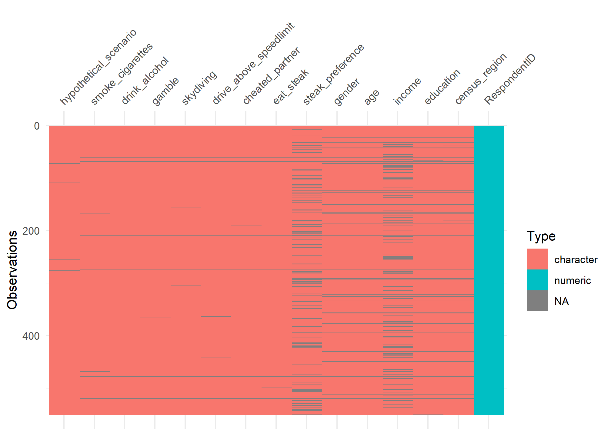
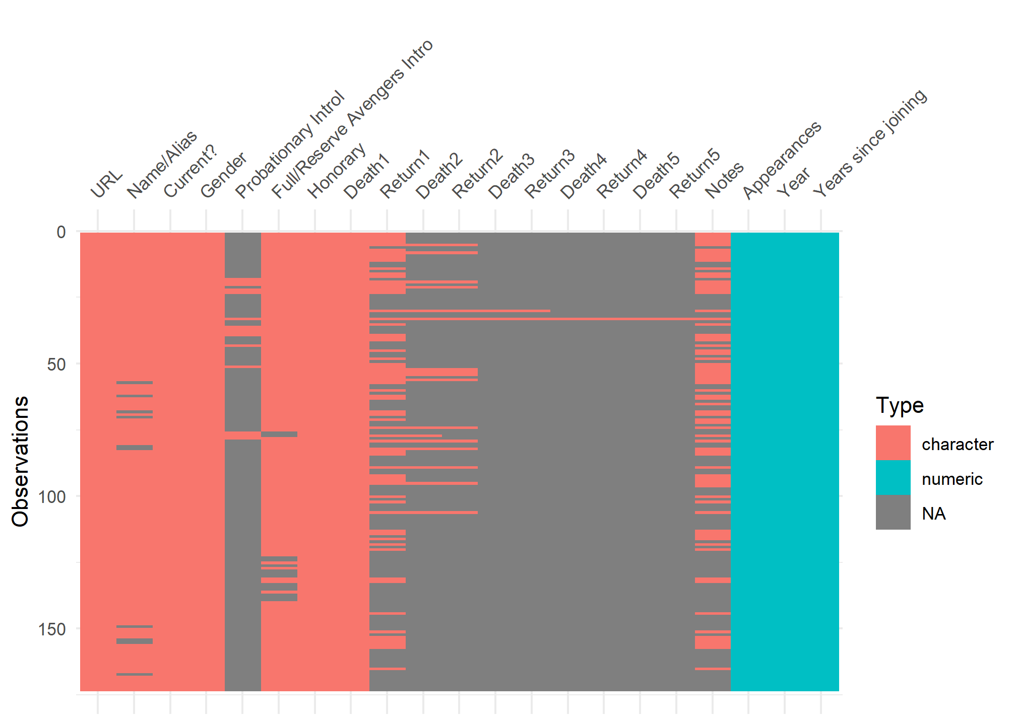
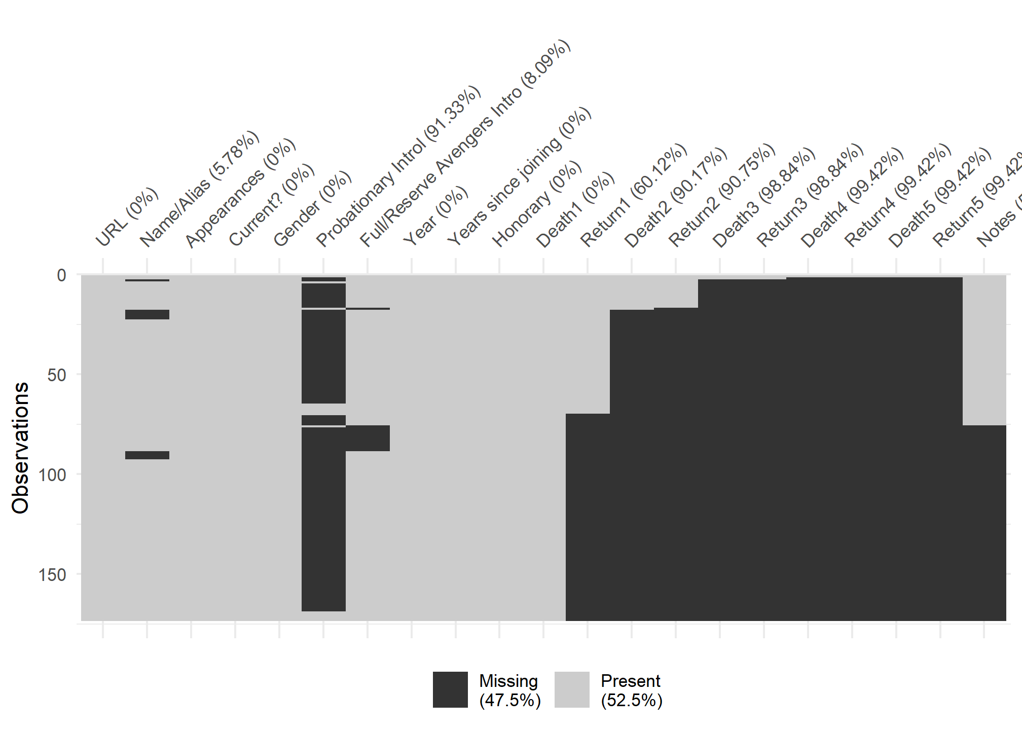
visdat:
![]()
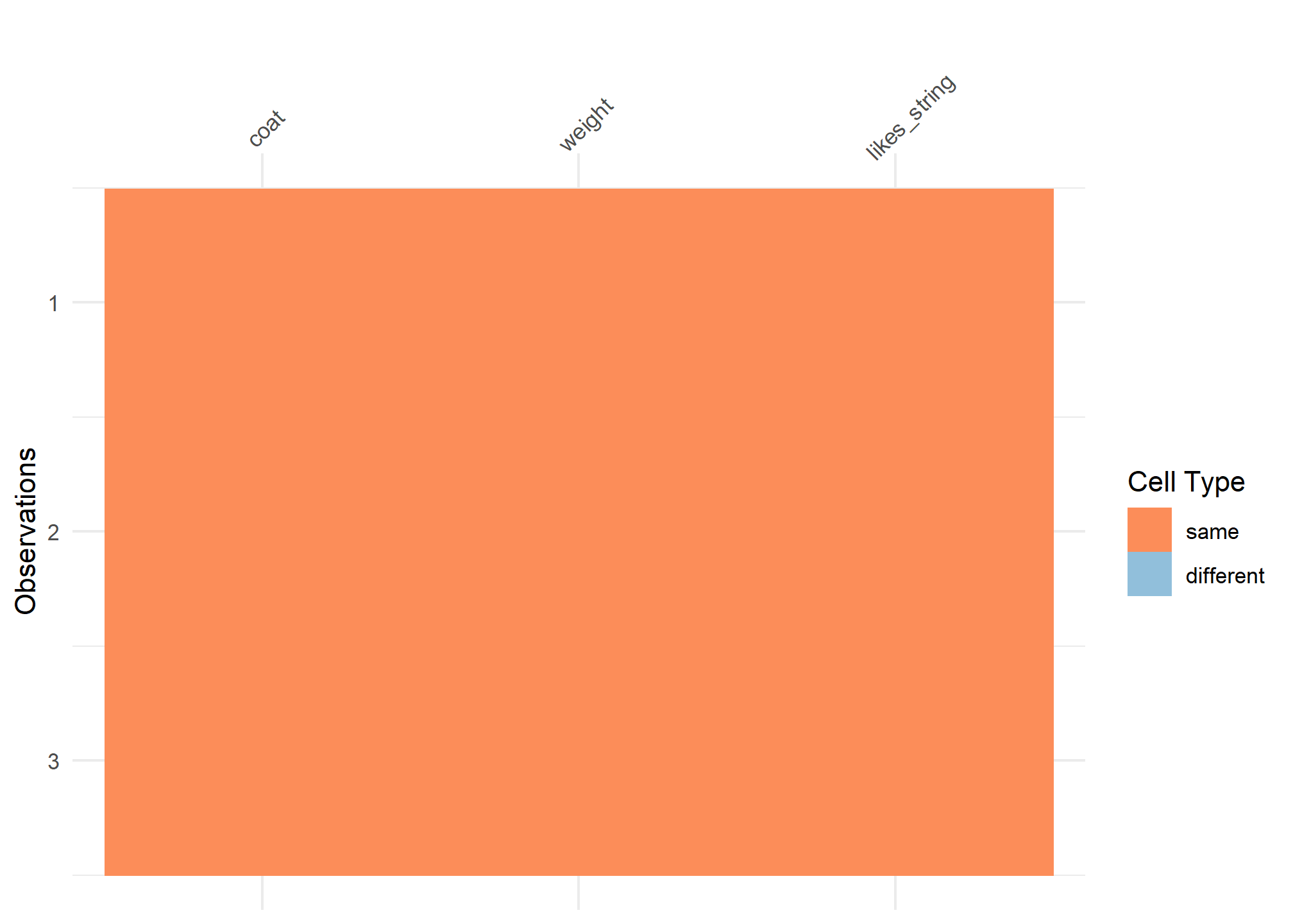
helps you visualise a dataframe and “get a look at the data” by displaying the variable classes in a dataframe as a plot with vis_dat, and getting a brief look into missing data patterns using vis_miss.
# install.packages("visdat")
library(visdat)

#overall viz
vis_dat(steak)
vis_dat(avengers)
#missing viz
vis_miss(avengers,
         cluster = TRUE)
#comparison viz
vis_compare(cats_tibble, cats_tribble)
Why EDA
Why do we want to visualize our data?
- All the graphs are based on data with the same summary statistics!
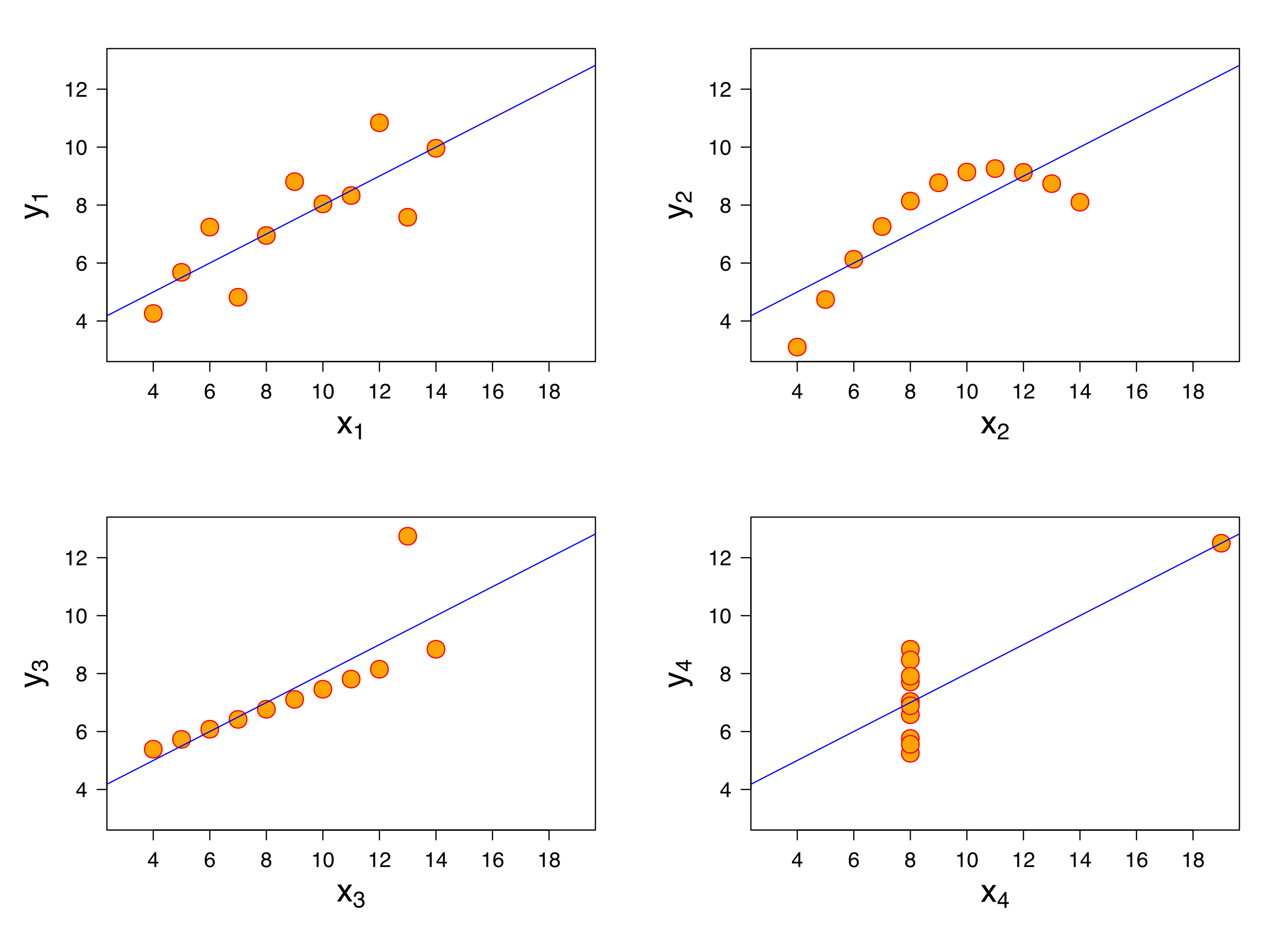
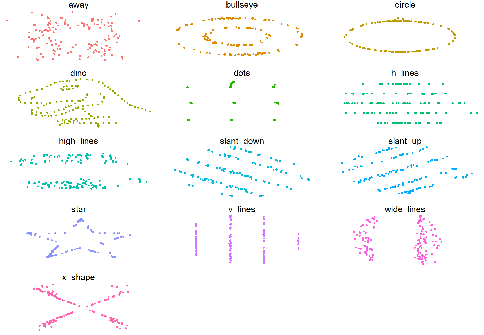
We can see this more explicitly with the “DatasauRus Dozen” Package. We have nearly identical summary statistics, but the actual data looks vastly different from eachother.
library(datasauRus)
datasaurus_dozen %>%
  group_by(dataset) %>%
  summarize(
    mean_x    = mean(x),
    mean_y    = mean(y),
    std_dev_x = sd(x),
    std_dev_y = sd(y),
    corr_x_y  = cor(x, y)
  )
## # A tibble: 13 x 6
##    dataset    mean_x mean_y std_dev_x std_dev_y corr_x_y
##  * <chr>       <dbl>  <dbl>     <dbl>     <dbl>    <dbl>
##  1 away         54.3   47.8      16.8      26.9  -0.0641
##  2 bullseye     54.3   47.8      16.8      26.9  -0.0686
##  3 circle       54.3   47.8      16.8      26.9  -0.0683
##  4 dino         54.3   47.8      16.8      26.9  -0.0645
##  5 dots         54.3   47.8      16.8      26.9  -0.0603
##  6 h_lines      54.3   47.8      16.8      26.9  -0.0617
##  7 high_lines   54.3   47.8      16.8      26.9  -0.0685
##  8 slant_down   54.3   47.8      16.8      26.9  -0.0690
##  9 slant_up     54.3   47.8      16.8      26.9  -0.0686
## 10 star         54.3   47.8      16.8      26.9  -0.0630
## 11 v_lines      54.3   47.8      16.8      26.9  -0.0694
## 12 wide_lines   54.3   47.8      16.8      26.9  -0.0666
## 13 x_shape      54.3   47.8      16.8      26.9  -0.0656
ggplot(datasaurus_dozen,
       aes(x=x, y=y, color=dataset))+
  geom_point(size = .5)+
  theme_void()+
  theme(legend.position = "none")+
  facet_wrap(~dataset, ncol=3)
Data Export
write_csv(), write_csv2(), and write_tsv()
- You can write comma-separated and tab-separated files using
write_csv(),write_csv2(), andwrite_tsv().
steak %>%
  filter(hypothetical_scenario == "Lottery B") %>%
  write_csv("../output/nyc_region_data.csv")
- The defaults are usually fine.
Reading/Writing R Objects with readRDS() and saveRDS().
- You can save and reload arbitrary R objects (data frames, matrices, lists,
vectors) using
readRDS()andsaveRDS(). - .Rds files are compressed data files so enable much faster loading and more compact storage. - These are what usually go into the /data folder as opposed to the /data_raw folder
steak %>%
  filter(hypothetical_scenario == "Lottery B") %>%
  saveRDS("../output/nyc_region_data.rds")
References
- Chapter 11 of RDS
- Chapter 7 of RDS
- Data Import Cheatsheet
- Readr Overview
- Haven Documentation
- readxl Documentation
-
“The Datasaurus Data Package,” accessed September 16, 2019, https://cran.r-project.org/web/packages/datasauRus/vignettes/Datasaurus.html. ↩︎