Relational Data and Joins

Content for week of Monday, March 15, 2021–Thursday, March 18, 2021

Learning Outcomes

Describe relational data.
Use the correct R tidyverse function to manipulate data:
- inner_join(),
- left_join(),
- right_join(),
- full_join(),
- semi_join(),
- anti_join().

Relational Data

Load the tidyverse

library(tidyverse)

Many datasets (especially those drawn from relational databases) have more than two data frames.
These data frames are often logically related where rows in one data frame correspond to, or, have a relation to, rows in another data frame.
Large Relational Databases are typically designed (by data engineers) to achieve some level of “normalization”
The goal of normalization is to design the set of tables (data frames) to capture all of the data while achieving a balance across:
- storage size,
- query speed,
- ease of maintenance by users, and
- minimal delays for distributed operations with multiple users.
Table design strives to:
- reduce data duplication (which increases storage and the potential for errors), and
- enable multiple users to update their tables without interference from other users.
A principle of normalization is to limit tables to a single purpose.
As R users, we might say, a table (dataframe) describes one type of (observational or experimental) unit, with all the observations for each variable associated with that unit and only that unit.
In modern databases, you may run into tables containing blob objects such as pictures, figures, or movies
- You may need to work with the database administrator to get only the data you need into R.

Example: The Lahman Data Set has Multiple Tables

Consider the tables/data frames in the lahman package.

install.packages("Lahman")

library(Lahman)

Use the data(package = "package-name") to see the data sets in a package

data(package = "Lahman")

Each Table has One Purpose: To Describe One Type of Unit

# Let's turn these 5 dataframes into tibbles while we're here:
People <- as_tibble(Lahman::People)
Teams <- as_tibble(Lahman::Teams)
Fielding <- as_tibble(Lahman::Fielding)
Pitching <- as_tibble(Lahman::Pitching)
Batting <- as_tibble(Lahman::Batting)


# `People`: Player names, DOB, and biographical info.
head(People)

## # A tibble: 6 x 26
##   playerID birthYear birthMonth birthDay birthCountry birthState birthCity
##   <chr>        <int>      <int>    <int> <chr>        <chr>      <chr>    
## 1 aardsda~      1981         12       27 USA          CO         Denver   
## 2 aaronha~      1934          2        5 USA          AL         Mobile   
## 3 aaronto~      1939          8        5 USA          AL         Mobile   
## 4 aasedo01      1954          9        8 USA          CA         Orange   
## 5 abadan01      1972          8       25 USA          FL         Palm Bea~
## 6 abadfe01      1985         12       17 D.R.         La Romana  La Romana
## # ... with 19 more variables: deathYear <int>, deathMonth <int>,
## #   deathDay <int>, deathCountry <chr>, deathState <chr>, deathCity <chr>,
## #   nameFirst <chr>, nameLast <chr>, nameGiven <chr>, weight <int>,
## #   height <int>, bats <fct>, throws <fct>, debut <chr>, finalGame <chr>,
## #   retroID <chr>, bbrefID <chr>, deathDate <date>, birthDate <date>

# `Teams`: Yearly statistics and standings for teams.
head(Teams)

## # A tibble: 6 x 48
##   yearID lgID  teamID franchID divID  Rank     G Ghome     W     L DivWin WCWin
##    <int> <fct> <fct>  <fct>    <chr> <int> <int> <int> <int> <int> <chr>  <chr>
## 1   1871 NA    BS1    BNA      <NA>      3    31    NA    20    10 <NA>   <NA> 
## 2   1871 NA    CH1    CNA      <NA>      2    28    NA    19     9 <NA>   <NA> 
## 3   1871 NA    CL1    CFC      <NA>      8    29    NA    10    19 <NA>   <NA> 
## 4   1871 NA    FW1    KEK      <NA>      7    19    NA     7    12 <NA>   <NA> 
## 5   1871 NA    NY2    NNA      <NA>      5    33    NA    16    17 <NA>   <NA> 
## 6   1871 NA    PH1    PNA      <NA>      1    28    NA    21     7 <NA>   <NA> 
## # ... with 36 more variables: LgWin <chr>, WSWin <chr>, R <int>, AB <int>,
## #   H <int>, X2B <int>, X3B <int>, HR <int>, BB <int>, SO <int>, SB <int>,
## #   CS <int>, HBP <int>, SF <int>, RA <int>, ER <int>, ERA <dbl>, CG <int>,
## #   SHO <int>, SV <int>, IPouts <int>, HA <int>, HRA <int>, BBA <int>,
## #   SOA <int>, E <int>, DP <int>, FP <dbl>, name <chr>, park <chr>,
## #   attendance <int>, BPF <int>, PPF <int>, teamIDBR <chr>,
## #   teamIDlahman45 <chr>, teamIDretro <chr>

# `Fielding`: Fielding stats
head(Fielding)

## # A tibble: 6 x 18
##   playerID yearID stint teamID lgID  POS       G    GS InnOuts    PO     A     E
##   <chr>     <int> <int> <fct>  <fct> <chr> <int> <int>   <int> <int> <int> <int>
## 1 abercda~   1871     1 TRO    NA    SS        1     1      24     1     3     2
## 2 addybo01   1871     1 RC1    NA    2B       22    22     606    67    72    42
## 3 addybo01   1871     1 RC1    NA    SS        3     3      96     8    14     7
## 4 allisar~   1871     1 CL1    NA    2B        2     0      18     1     4     0
## 5 allisar~   1871     1 CL1    NA    OF       29    29     729    51     3     7
## 6 allisdo~   1871     1 WS3    NA    C        27    27     681    68    15    20
## # ... with 6 more variables: DP <int>, PB <int>, WP <int>, SB <int>, CS <int>,
## #   ZR <int>

# `Pitching`: Pitching stats
head(Pitching)

## # A tibble: 6 x 30
##   playerID yearID stint teamID lgID      W     L     G    GS    CG   SHO    SV
##   <chr>     <int> <int> <fct>  <fct> <int> <int> <int> <int> <int> <int> <int>
## 1 bechtge~   1871     1 PH1    NA        1     2     3     3     2     0     0
## 2 brainas~   1871     1 WS3    NA       12    15    30    30    30     0     0
## 3 fergubo~   1871     1 NY2    NA        0     0     1     0     0     0     0
## 4 fishech~   1871     1 RC1    NA        4    16    24    24    22     1     0
## 5 fleetfr~   1871     1 NY2    NA        0     1     1     1     1     0     0
## 6 flowedi~   1871     1 TRO    NA        0     0     1     0     0     0     0
## # ... with 18 more variables: IPouts <int>, H <int>, ER <int>, HR <int>,
## #   BB <int>, SO <int>, BAOpp <dbl>, ERA <dbl>, IBB <int>, WP <int>, HBP <int>,
## #   BK <int>, BFP <int>, GF <int>, R <int>, SH <int>, SF <int>, GIDP <int>

# `Batting`: Batting stats
head(Batting)

## # A tibble: 6 x 22
##   playerID yearID stint teamID lgID      G    AB     R     H   X2B   X3B    HR
##   <chr>     <int> <int> <fct>  <fct> <int> <int> <int> <int> <int> <int> <int>
## 1 abercda~   1871     1 TRO    NA        1     4     0     0     0     0     0
## 2 addybo01   1871     1 RC1    NA       25   118    30    32     6     0     0
## 3 allisar~   1871     1 CL1    NA       29   137    28    40     4     5     0
## 4 allisdo~   1871     1 WS3    NA       27   133    28    44    10     2     2
## 5 ansonca~   1871     1 RC1    NA       25   120    29    39    11     3     0
## 6 armstbo~   1871     1 FW1    NA       12    49     9    11     2     1     0
## # ... with 10 more variables: RBI <int>, SB <int>, CS <int>, BB <int>,
## #   SO <int>, IBB <int>, HBP <int>, SH <int>, SF <int>, GIDP <int>

These Tables are Logically Connected

Fields in one table “relate” to fields in one or more other tables

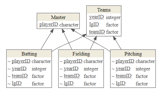
For Lahman:
- Batting, Fielding, and Pitching connect to People via a single variable, PeopleID.
- Batting, Fielding, and Pitching connect to Teams through the YearID, TeamID and lgID variables.

We Define Variables as “Keys” to Identify Rows and to Make Logical Connections Between Tables.

Every Table should have a Primary key to uniquely identify (differentiate) its rows.
- Keys must be unique in their own table, i,e., only refer to one instance of an item.
- Good Data engineers create keys with no intrinsic meaning other than being a unique identifier.
- Some tables may use a combined key based on multiple columns, e.g., year, month, day together.
- The primary key from one table may appear many times in other tables.
Example: People$playerID is a primary key for People because it uniquely identifies the rows in People.
To check if you have identified the Primary Key fields, use group_by(primary_key_fields) and count() to see if there are multiple rows for any group.
If any group has more than one row, the fields are insufficient to serve as a primary key

# type is Not a Primary Key
People %>%
  group_by(nameLast) %>%
  count() %>%
  filter(n > 1)

## # A tibble: 2,559 x 2
## # Groups:   nameLast [2,559]
##    nameLast        n
##    <chr>       <int>
##  1 Aaron           2
##  2 Abad            2
##  3 Abbey           2
##  4 Abbott          9
##  5 Abercrombie     2
##  6 Abernathy       4
##  7 Abrams          2
##  8 Abreu           7
##  9 Acevedo         2
## 10 Acker           2
## # ... with 2,549 more rows

# This is a primary key
People %>%
  group_by(playerID) %>%
  count() %>%
  filter(n > 1)

## # A tibble: 0 x 2
## # Groups:   playerID [0]
## # ... with 2 variables: playerID <chr>, n <int>

A primary key can also serve as a foreign key when present in another table.
A Foreign key is used to identify rows in another (child) table.
Example: In Pitching, $playerID is a foreign key for the other table People because it uniquely identifies rows in People.
There can be multiple rows with the same foreign key in a table, e.g., playerID in Pitching, so Pitching$playerID is not a primary key in Pitching

Pitching %>% 
  group_by(playerID) %>%
  count() %>%
  filter(n > 1)

## # A tibble: 6,980 x 2
## # Groups:   playerID [6,980]
##    playerID      n
##    <chr>     <int>
##  1 aardsda01     9
##  2 aasedo01     13
##  3 abadfe01     10
##  4 abbeybe01     6
##  5 abbotgl01    12
##  6 abbotji01    11
##  7 abbotky01     4
##  8 abbotpa01    12
##  9 aberal01      8
## 10 abernte01     3
## # ... with 6,970 more rows

Join Functions in the dplyr Package

Getting data from two (or more) tables requires using the primary keys and foreign keys to logically connect the tables.
These “connections” are called joins
The dplyr package has functions to connect or join tables so you can work with their data
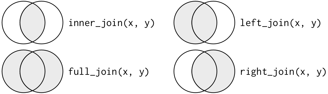
The dplyr package supports seven types of joins:
- Four types of mutating joins,
- Two types of filtering joins, and
- A nesting join.
Many sources refer to the first table in a join function argument list as the x table or the left table or the “parent” table and second table in the argument as the y table or the right table or the “child” table
The primary key fields for the y/right/child table must be able to be matched to fields in the x/left/parent table which can serve as a foreign key.

Mutating Joins: Inner, Left, Right, Full

Mutating Joins affect the rows and columns of either the x or y table
inner_join(): returns all rows from x where there are matching values in y, and all columns from x and y.

If there are multiple matches between x and y, all combination of the matches are returned.
Rows that do not match are not returned

left_join():returns all rows from x, and all columns from x and y.

Rows in x with no match in y are returned but will have NA values in the new columns.
If there are multiple matches between x and y, all combinations of the matches are returned.

right_join(): returns all rows from y, and all columns from x and y.

Rows in y with no match in x will have NA values in the new columns.
If there are multiple matches between x and y, all combinations of the matches are returned.

full_join(): returns all rows and all columns from both x and y.

Where there are not matching values, returns NA for the missing values.

x <- tribble(
  ~key, ~val_x,
     1, "x1",
     2, "x2",
     3, "x3"
)
x

## # A tibble: 3 x 2
##     key val_x
##   <dbl> <chr>
## 1     1 x1   
## 2     2 x2   
## 3     3 x3

y <- tribble(
  ~key, ~val_y,
     1, "y1",
     2, "y2",
     4, "y4"
)
y

## # A tibble: 3 x 2
##     key val_y
##   <dbl> <chr>
## 1     1 y1   
## 2     2 y2   
## 3     4 y4

`inner_join(x, y)`

This is the simplest join to add
Matches the rows of x with rows of y only when their keys are equal.

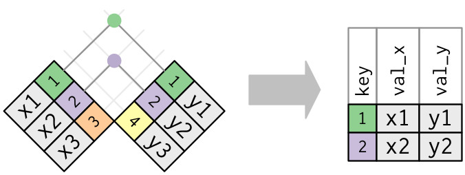
inner_join(x, y, by = "key")

## # A tibble: 2 x 3
##     key val_x val_y
##   <dbl> <chr> <chr>
## 1     1 x1    y1   
## 2     2 x2    y2

Keeps all rows that appear in both data frames.
if the key is missing on either the left or right side, that row will be dropped from the join.

Exercise:

Select all batting stats for players who were born in the 1980s.

People %>% 
  filter(between(birthYear, 1980, 1989)) %>% 
  nrow()

## [1] 2207

nrow(Batting)

## [1] 107429

People %>% 
  filter(between(birthYear, 1980, 1989)) %>% 
  inner_join(Batting, by = "playerID") %>% 
  nrow()

## [1] 12516

Outer Joins: Left, Right, Full

Outer Joins keep all rows that appear in at least one data frame and add columns from the other table for those rows.

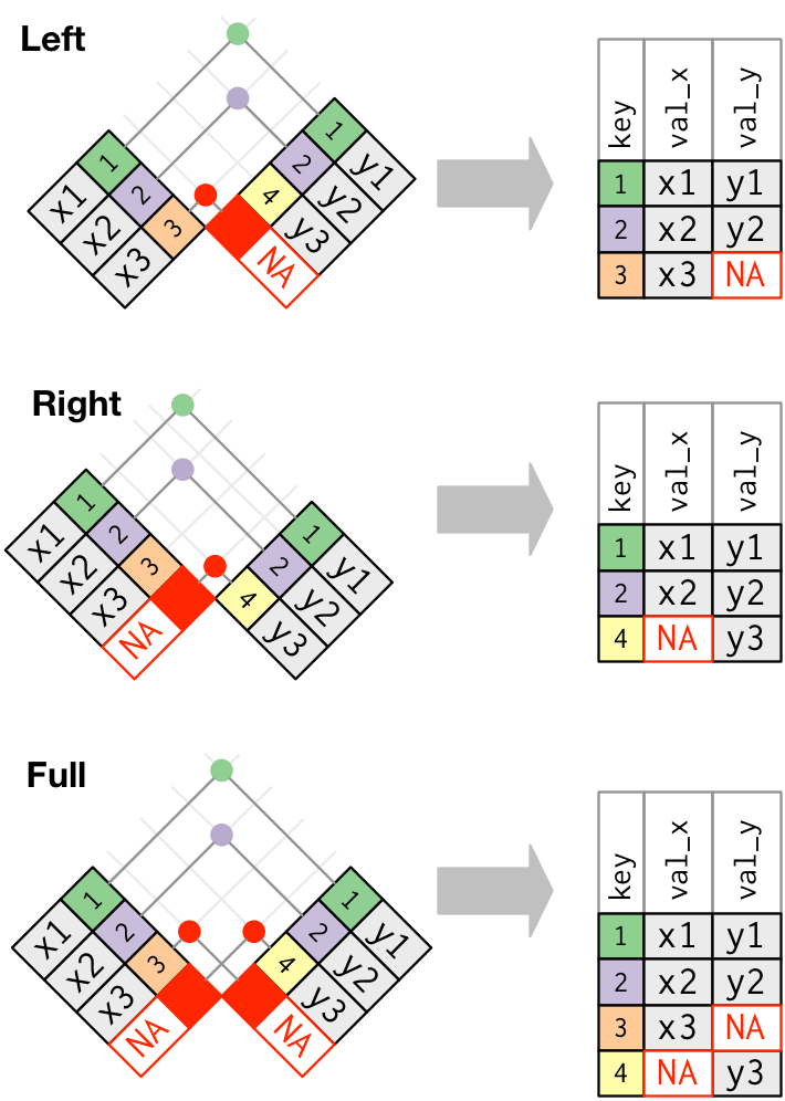
`left_join(x, y)`

Keeps all rows of x and adds columns from y.
Puts in NA in the new y columns if no match.
By far the most common join
Always use a left join unless you have a good reason not to.

left_join(x, y, by = "key")

## # A tibble: 3 x 3
##     key val_x val_y
##   <dbl> <chr> <chr>
## 1     1 x1    y1   
## 2     2 x2    y2   
## 3     3 x3    <NA>

`right_join(x, y)`

Keeps all rows of yand adds columns from x.
Puts in NA in x columns if no match.

right_join(x, y, by = "key")

## # A tibble: 3 x 3
##     key val_x val_y
##   <dbl> <chr> <chr>
## 1     1 x1    y1   
## 2     2 x2    y2   
## 3     4 <NA>  y4

Note what happens when you switch the type of join and the data frame

left_join(y, x, by = "key")

## # A tibble: 3 x 3
##     key val_y val_x
##   <dbl> <chr> <chr>
## 1     1 y1    x1   
## 2     2 y2    x2   
## 3     4 y4    <NA>

You have flexibility to choose the order you are doing the joins and the type of joins to get the results you want from your workflow.

`full_join(x, y)`

Keeps all rows of both and adds columns from y to x.
Puts in NA wherever there is no match
Can cause a lot of extra rows and columns with NAs if not careful
Only use when absolutely necessary and then only after you have selected the desired variables and filtered the desired rows.

full_join(x, y, by = "key")

## # A tibble: 4 x 3
##     key val_x val_y
##   <dbl> <chr> <chr>
## 1     1 x1    y1   
## 2     2 x2    y2   
## 3     3 x3    <NA> 
## 4     4 <NA>  y4

Exercise:

Add the team name to the Batting data frame.

names(Batting)

##  [1] "playerID" "yearID"   "stint"    "teamID"   "lgID"     "G"       
##  [7] "AB"       "R"        "H"        "X2B"      "X3B"      "HR"      
## [13] "RBI"      "SB"       "CS"       "BB"       "SO"       "IBB"     
## [19] "HBP"      "SH"       "SF"       "GIDP"

names(Teams)

##  [1] "yearID"         "lgID"           "teamID"         "franchID"      
##  [5] "divID"          "Rank"           "G"              "Ghome"         
##  [9] "W"              "L"              "DivWin"         "WCWin"         
## [13] "LgWin"          "WSWin"          "R"              "AB"            
## [17] "H"              "X2B"            "X3B"            "HR"            
## [21] "BB"             "SO"             "SB"             "CS"            
## [25] "HBP"            "SF"             "RA"             "ER"            
## [29] "ERA"            "CG"             "SHO"            "SV"            
## [33] "IPouts"         "HA"             "HRA"            "BBA"           
## [37] "SOA"            "E"              "DP"             "FP"            
## [41] "name"           "park"           "attendance"     "BPF"           
## [45] "PPF"            "teamIDBR"       "teamIDlahman45" "teamIDretro"

Batting %>% 
  left_join(Teams, by = "teamID") %>%
  select(name, everything())

## # A tibble: 8,699,563 x 69
##    name  playerID yearID.x stint teamID lgID.x   G.x  AB.x   R.x   H.x X2B.x
##    <chr> <chr>       <int> <int> <fct>  <fct>  <int> <int> <int> <int> <int>
##  1 Troy~ abercda~     1871     1 TRO    NA         1     4     0     0     0
##  2 Troy~ abercda~     1871     1 TRO    NA         1     4     0     0     0
##  3 Rock~ addybo01     1871     1 RC1    NA        25   118    30    32     6
##  4 Clev~ allisar~     1871     1 CL1    NA        29   137    28    40     4
##  5 Clev~ allisar~     1871     1 CL1    NA        29   137    28    40     4
##  6 Wash~ allisdo~     1871     1 WS3    NA        27   133    28    44    10
##  7 Wash~ allisdo~     1871     1 WS3    NA        27   133    28    44    10
##  8 Rock~ ansonca~     1871     1 RC1    NA        25   120    29    39    11
##  9 Fort~ armstbo~     1871     1 FW1    NA        12    49     9    11     2
## 10 Rock~ barkeal~     1871     1 RC1    NA         1     4     0     1     0
## # ... with 8,699,553 more rows, and 58 more variables: X3B.x <int>, HR.x <int>,
## #   RBI <int>, SB.x <int>, CS.x <int>, BB.x <int>, SO.x <int>, IBB <int>,
## #   HBP.x <int>, SH <int>, SF.x <int>, GIDP <int>, yearID.y <int>,
## #   lgID.y <fct>, franchID <fct>, divID <chr>, Rank <int>, G.y <int>,
## #   Ghome <int>, W <int>, L <int>, DivWin <chr>, WCWin <chr>, LgWin <chr>,
## #   WSWin <chr>, R.y <int>, AB.y <int>, H.y <int>, X2B.y <int>, X3B.y <int>,
## #   HR.y <int>, BB.y <int>, SO.y <int>, SB.y <int>, CS.y <int>, HBP.y <int>,
## #   SF.y <int>, RA <int>, ER <int>, ERA <dbl>, CG <int>, SHO <int>, SV <int>,
## #   IPouts <int>, HA <int>, HRA <int>, BBA <int>, SOA <int>, E <int>, DP <int>,
## #   FP <dbl>, park <chr>, attendance <int>, BPF <int>, PPF <int>,
## #   teamIDBR <chr>, teamIDlahman45 <chr>, teamIDretro <chr>

list the first name, last name, and team name for every player who played in 2018

Batting %>% 
  filter(yearID == 2018) %>% 
  left_join(People, by = "playerID") %>% 
  left_join(Teams, by = "teamID") %>% 
  select(nameFirst, nameLast, name) %>% 
  distinct()

## # A tibble: 2,426 x 3
##    nameFirst nameLast name                
##    <chr>     <chr>    <chr>               
##  1 Jose      Abreu    Chicago White Sox   
##  2 Ronald    Acuna    Atlanta Braves      
##  3 Willy     Adames   Tampa Bay Devil Rays
##  4 Willy     Adames   Tampa Bay Rays      
##  5 Jason     Adam     Kansas City Royals  
##  6 Austin    Adams    Washington Senators 
##  7 Austin    Adams    Washington Nationals
##  8 Chance    Adams    New York Highlanders
##  9 Chance    Adams    New York Yankees    
## 10 Lane      Adams    Atlanta Braves      
## # ... with 2,416 more rows

Duplicate Keys

One would not expect to have rows with duplicate primary keys in a table from a relational database (most enforce no duplicates on the primary key fields)
However, data from sources without rules enforcing key uniqueness often have them.
If you have duplicate keys the x table, then during a left join with a y where there is no duplication, the rows of y are copied multiple times into the new x data frame.

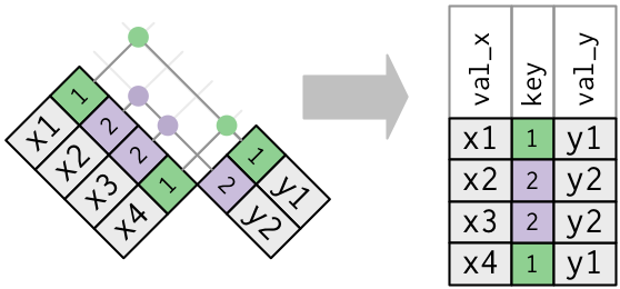
This can be useful when you want to add additional information (rows) to x as there can be a one-to-many relationship.
In a sense the “original” x key was really a foreign key with respect to the join as it did not uniquely identify the rows in x but was a primary key for y.

x_mult <- tribble(~key, ~val_x,
                  ##--  ------
                  1,    "x1",
                  2,    "x2",
                  2,    "x3",
                  1,    "x4")
y

## # A tibble: 3 x 2
##     key val_y
##   <dbl> <chr>
## 1     1 y1   
## 2     2 y2   
## 3     4 y4

x_mult %>% 
  left_join(y, by = "key")

## # A tibble: 4 x 3
##     key val_x val_y
##   <dbl> <chr> <chr>
## 1     1 x1    y1   
## 2     2 x2    y2   
## 3     2 x3    y2   
## 4     1 x4    y1

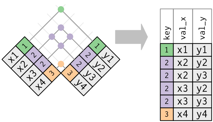
If you have duplicate keys in both (usually a mistake), then you get every possible combination of the values in x and y at the key values where there are duplications.

x_mult

## # A tibble: 4 x 2
##     key val_x
##   <dbl> <chr>
## 1     1 x1   
## 2     2 x2   
## 3     2 x3   
## 4     1 x4

y_mult <- tribble(~key, ~val_y,
                  ##--  ------
                  1,    "y1",
                  2,    "y2",
                  2,    "y3",
                  1,    "y4")

left_join(x_mult, y_mult, by = "key")

## # A tibble: 8 x 3
##     key val_x val_y
##   <dbl> <chr> <chr>
## 1     1 x1    y1   
## 2     1 x1    y4   
## 3     2 x2    y2   
## 4     2 x2    y3   
## 5     2 x3    y2   
## 6     2 x3    y3   
## 7     1 x4    y1   
## 8     1 x4    y4

Filtering Joins Filter Rows in the Left (`x`) Data Frame:

They do not add columns; they just filter the rows of x based on values in y
semi_join(): returns all rows from x where there are matching key values in y, keeping just columns from x.
- Filters out rows in x that do not match anything in y.
A semi-join is not the same as an inner join
- an inner join will return one row of x for each matching row of y, (potentially adding multiple rows) whereas
- a semi-join will never duplicate rows of x.

`semi_join(x, y)`

Keeps all of the rows in x that have a match in y (but doesn’t add the variables of y to x).

semi_join(x, y, by = "key")

## # A tibble: 2 x 2
##     key val_x
##   <dbl> <chr>
## 1     1 x1   
## 2     2 x2

`anti_join()`

anti_join(): returns all rows from x where there are not matching key values in y, keeping just columns from x.
- Filters out rows in x that do match anything in y (the rows with no join).
Drops all of the rows in x that do not have a match in y (but doesn’t add the variables of y to x).

In human speak, what’s in x but not y?

anti_join(x, y, by = "key")

## # A tibble: 1 x 2
##     key val_x
##   <dbl> <chr>
## 1     3 x3

Exercise:

Find the 10 players with the highest number of strikeouts (SO) from the Batting table and assign to a new data frame.
Join the appropriate data frames to select all players from those 10 days.

ten_worst <- Batting %>%
  group_by(playerID) %>%
  summarize(count_strikeout = sum(SO, na.rm = TRUE)) %>%
  slice_max(count_strikeout, n =10) 

People %>% 
  semi_join(ten_worst)

## # A tibble: 10 x 26
##    playerID birthYear birthMonth birthDay birthCountry birthState birthCity
##    <chr>        <int>      <int>    <int> <chr>        <chr>      <chr>    
##  1 cansejo~      1964          7        2 Cuba         La Habana  La Habana
##  2 dunnad01      1979         11        9 USA          TX         Houston  
##  3 galaran~      1961          6       18 Venezuela    Distrito ~ Caracas  
##  4 grandcu~      1981          3       16 USA          IL         Blue Isl~
##  5 jacksre~      1946          5       18 USA          PA         Abington 
##  6 reynoma~      1983          8        3 USA          KY         Pikeville
##  7 rodrial~      1975          7       27 USA          NY         New York 
##  8 sosasa01      1968         11       12 D.R.         San Pedro~ San Pedr~
##  9 stargwi~      1940          3        6 USA          OK         Earlsboro
## 10 thomeji~      1970          8       27 USA          IL         Peoria   
## # ... with 19 more variables: deathYear <int>, deathMonth <int>,
## #   deathDay <int>, deathCountry <chr>, deathState <chr>, deathCity <chr>,
## #   nameFirst <chr>, nameLast <chr>, nameGiven <chr>, weight <int>,
## #   height <int>, bats <fct>, throws <fct>, debut <chr>, finalGame <chr>,
## #   retroID <chr>, bbrefID <chr>, deathDate <date>, birthDate <date>

#note, you can do this same operation with filtering too:
    ten_worst_vector <- ten_worst %>% 
      pull(playerID)
    
    People %>% 
      filter(playerID %in% ten_worst_vector)

## # A tibble: 10 x 26
##    playerID birthYear birthMonth birthDay birthCountry birthState birthCity
##    <chr>        <int>      <int>    <int> <chr>        <chr>      <chr>    
##  1 cansejo~      1964          7        2 Cuba         La Habana  La Habana
##  2 dunnad01      1979         11        9 USA          TX         Houston  
##  3 galaran~      1961          6       18 Venezuela    Distrito ~ Caracas  
##  4 grandcu~      1981          3       16 USA          IL         Blue Isl~
##  5 jacksre~      1946          5       18 USA          PA         Abington 
##  6 reynoma~      1983          8        3 USA          KY         Pikeville
##  7 rodrial~      1975          7       27 USA          NY         New York 
##  8 sosasa01      1968         11       12 D.R.         San Pedro~ San Pedr~
##  9 stargwi~      1940          3        6 USA          OK         Earlsboro
## 10 thomeji~      1970          8       27 USA          IL         Peoria   
## # ... with 19 more variables: deathYear <int>, deathMonth <int>,
## #   deathDay <int>, deathCountry <chr>, deathState <chr>, deathCity <chr>,
## #   nameFirst <chr>, nameLast <chr>, nameGiven <chr>, weight <int>,
## #   height <int>, bats <fct>, throws <fct>, debut <chr>, finalGame <chr>,
## #   retroID <chr>, bbrefID <chr>, deathDate <date>, birthDate <date>

Other Key Names

If the primary and foreign keys names do not match, you need to specify the matching names in a vector
Example: left_join(x, y, by = c("a" = "b")), where a is the key in x and b is the key in y.
Here we join by single keys with different names in the x and y data frames

library(nycflights13)
flights %>% 
  left_join(airports, by = c("origin" = "faa")) %>% 
  head()

## # A tibble: 6 x 26
##    year month   day dep_time sched_dep_time dep_delay arr_time sched_arr_time
##   <int> <int> <int>    <int>          <int>     <dbl>    <int>          <int>
## 1  2013     1     1      517            515         2      830            819
## 2  2013     1     1      533            529         4      850            830
## 3  2013     1     1      542            540         2      923            850
## 4  2013     1     1      544            545        -1     1004           1022
## 5  2013     1     1      554            600        -6      812            837
## 6  2013     1     1      554            558        -4      740            728
## # ... with 18 more variables: arr_delay <dbl>, carrier <chr>, flight <int>,
## #   tailnum <chr>, origin <chr>, dest <chr>, air_time <dbl>, distance <dbl>,
## #   hour <dbl>, minute <dbl>, time_hour <dttm>, name <chr>, lat <dbl>,
## #   lon <dbl>, alt <dbl>, tz <dbl>, dst <chr>, tzone <chr>

If you have multiple variables acting as a combined key, specify the by argument as a vector.
If they have the same name, you can drop the = argument
The , serve as an “AND” operator

Fielding %>% 
left_join(Teams, by = c("yearID", "lgID", "teamID")) %>% 
  head()

## # A tibble: 6 x 63
##   playerID yearID stint teamID lgID  POS     G.x    GS InnOuts    PO     A   E.x
##   <chr>     <int> <int> <fct>  <fct> <chr> <int> <int>   <int> <int> <int> <int>
## 1 abercda~   1871     1 TRO    NA    SS        1     1      24     1     3     2
## 2 addybo01   1871     1 RC1    NA    2B       22    22     606    67    72    42
## 3 addybo01   1871     1 RC1    NA    SS        3     3      96     8    14     7
## 4 allisar~   1871     1 CL1    NA    2B        2     0      18     1     4     0
## 5 allisar~   1871     1 CL1    NA    OF       29    29     729    51     3     7
## 6 allisdo~   1871     1 WS3    NA    C        27    27     681    68    15    20
## # ... with 51 more variables: DP.x <int>, PB <int>, WP <int>, SB.x <int>,
## #   CS.x <int>, ZR <int>, franchID <fct>, divID <chr>, Rank <int>, G.y <int>,
## #   Ghome <int>, W <int>, L <int>, DivWin <chr>, WCWin <chr>, LgWin <chr>,
## #   WSWin <chr>, R <int>, AB <int>, H <int>, X2B <int>, X3B <int>, HR <int>,
## #   BB <int>, SO <int>, SB.y <int>, CS.y <int>, HBP <int>, SF <int>, RA <int>,
## #   ER <int>, ERA <dbl>, CG <int>, SHO <int>, SV <int>, IPouts <int>, HA <int>,
## #   HRA <int>, BBA <int>, SOA <int>, E.y <int>, DP.y <int>, FP <dbl>,
## #   name <chr>, park <chr>, attendance <int>, BPF <int>, PPF <int>,
## #   teamIDBR <chr>, teamIDlahman45 <chr>, teamIDretro <chr>

You can specify both multiple variables and with different names if necessary
You cannot specify one key from x to have two different values in y - there is no “OR” operation; you have to do two joins.

Set operations

{width = 50%}

x <- tribble(
  ~key, ~val,
     1, "a",
     1, "b",
     2, "a"
)

y <- tribble(
  ~key, ~val,
     1, "a",
     2, "b",
)

Set operations are occasionally useful when you want to break a single complex filter into simpler pieces. All these operations work with a complete row, comparing the values of every variable. These expect the x and y inputs to have the same variables, and treat the observations like sets.

Union

All unique rows from x and y.

union(y, x)

## # A tibble: 4 x 2
##     key val  
##   <dbl> <chr>
## 1     1 a    
## 2     2 b    
## 3     1 b    
## 4     2 a

intersect

Common rows in both x and y, keeping just unique rows.

intersect(x, y)

## # A tibble: 1 x 2
##     key val  
##   <dbl> <chr>
## 1     1 a

because table x had a dupicated row, it was removed.

setdiff

All rows from x which are not also rows in y, keeping just unique rows.

#what is in x but not in y?
setdiff(x, y)

## # A tibble: 2 x 2
##     key val  
##   <dbl> <chr>
## 1     1 b    
## 2     2 a

#what is in y but not in x?
setdiff(y, x)

## # A tibble: 1 x 2
##     key val  
##   <dbl> <chr>
## 1     2 b

Appending Data

Sometimes you want to add rows to your data instead of adding new columns. This happens a lot when you have new data coming in daily or weekly. To handle this data, we will use the bind_rows() function. To see how this works, let’s look at some play data about plant growth. In this situation, let’s say we have a sensor sending us new readings daily. How could we combine these data into one tibble?

march03 <- tibble::tribble(
             ~plant_id, ~treatment,     ~height, ~temperature,   ~humidity,
               "k3jak",  "control", 1.234156382,          82L, 0.257529979,
               "df33l",  "control", 1.380212809,          83L, 0.058794941,
               "l122j",  "treated", 1.526392762,          89L, 0.297541584,
               "3kssj",  "treated", 1.673373933,          80L, 0.881550707
             )


march04 <- tibble::tribble(
             ~plant_id, ~treatment,     ~height, ~temperature,   ~humidity,
               "k3jak",  "control", 1.660054506,          92L, 0.474884172,
               "df33l",  "control",  1.87979144,          83L, 0.769558459,
               "l122j",  "treated", 1.686950799,          86L, 0.228663423,
               "3kssj",  "treated", 2.032178067,          87L,   0.0340041
             )


march05 <- tibble::tribble(
             ~plant_id, ~treatment,     ~height, ~temperature,   ~humidity,
               "k3jak",  "control", 1.933533759,          89L, 0.975123013,
               "df33l",  "control", 1.990040605,          97L, 0.724627173,
               "l122j",  "treated", 1.996540851,          94L, 0.490475035,
               "3kssj",  "treated", 2.116540208,          93L, 0.169962639
             )

march03 <- march03 %>% 
  mutate(date = lubridate::mdy("03/03/2021"))
march04 <- march04 %>% 
  mutate(date = lubridate::mdy("03/04/2021"))
march05 <- march05 %>% 
  mutate(date = lubridate::mdy("03/05/2021"))

plants <- march03 %>% 
  bind_rows(march04) %>% 
  bind_rows(march05)

#alternatively, we could do a "subquery" on each of these dataframes.. 

march03 %>% 
  mutate(date = lubridate::mdy("03/03/2021")) %>% 
  bind_rows(mutate(march04, date = lubridate::mdy("03/04/2021"))) %>% 
  bind_rows(mutate(march05, date = lubridate::mdy("03/05/2021")))

## # A tibble: 12 x 6
##    plant_id treatment height temperature humidity date      
##    <chr>    <chr>      <dbl>       <int>    <dbl> <date>    
##  1 k3jak    control     1.23          82   0.258  2021-03-03
##  2 df33l    control     1.38          83   0.0588 2021-03-03
##  3 l122j    treated     1.53          89   0.298  2021-03-03
##  4 3kssj    treated     1.67          80   0.882  2021-03-03
##  5 k3jak    control     1.66          92   0.475  2021-03-04
##  6 df33l    control     1.88          83   0.770  2021-03-04
##  7 l122j    treated     1.69          86   0.229  2021-03-04
##  8 3kssj    treated     2.03          87   0.0340 2021-03-04
##  9 k3jak    control     1.93          89   0.975  2021-03-05
## 10 df33l    control     1.99          97   0.725  2021-03-05
## 11 l122j    treated     2.00          94   0.490  2021-03-05
## 12 3kssj    treated     2.12          93   0.170  2021-03-05

In the example above, why do we want to bind_rows() instead of a join?

Bind rows matches column names, so if there are missing columns, they will be filled with NA in the newly added rows like the following.

a <- tibble(x = 1:3, y = c(4,5,NA)) 
a

## # A tibble: 3 x 2
##       x     y
##   <int> <dbl>
## 1     1     4
## 2     2     5
## 3     3    NA

b <- tibble(y = 1:4, z = runif(4))
b

## # A tibble: 4 x 2
##       y     z
##   <int> <dbl>
## 1     1 0.177
## 2     2 0.198
## 3     3 0.801
## 4     4 0.550

a %>% 
  bind_rows(b)

## # A tibble: 7 x 3
##       x     y      z
##   <int> <dbl>  <dbl>
## 1     1     4 NA    
## 2     2     5 NA    
## 3     3    NA NA    
## 4    NA     1  0.177
## 5    NA     2  0.198
## 6    NA     3  0.801
## 7    NA     4  0.550

References

Chapter 13 of RDS.
Data Transformation Cheatsheet
TidyExplain GIFs
Lahman Database visualization code

Appendix on dbplyr

While we won’t dicuss this in the lecture, this is an important reference you will likely want for working with databases in R. Feel free to run through these exercises on your own time.

References
- Introduction to dbplyr

Motivation

R typically works with all of the data accessible in the working memory of your computer. The more memory the larger the data set you can work with.
In the era of big data there are many data set too large to fit into memory.
The dbplyr package allows R to work with “remote” on-disk data stored in a database.
This is particularly useful in two scenarios:
- Your data is already in a database on your computer or cloud drive as opposed to a .csv or rdata file.
- You have so much data it does not all fit into memory simultaneously and you need to use some external storage engine.
- If your data fits in memory, there is no advantage to putting it in a database: it will only be slower and more frustrating.

The dbplyr package

The dbplyr functions provide a common interface to a back-end package (DBI) so you can use dplyr functions with many different databases using the same code.
You need to install a specific back-end for the database type you want to connect to.
Five commonly used back-ends are:
- RSQLite embeds a SQLite database.
- RMariaDB connects to MySQL and MariaDB
- RPostgres connects to Postgres and Redshift.
- odbc connects to many commercial databases via the open database connectivity protocol (ODBC).
- bigrquery connects to Google’s BigQuery.

Structured Query Language (SQL)

SQL is a language used for many years to interact with data sets stored in relational database management systems (RDBMS).
Common actions include: select, insert, update, or delete individual records as well as the different kinds of joins across the tables in the RDBMS
The dbplyr package implements the most common actions people do with SQL (but SQL can do more).
As the database back-end for dplyr, dbplyr automatically converts dplyr code into SQL

Example using RSQLite with a soccer data set

We’ll use a soccer dataset with multiple tables to demonstrate how to use dbplyr (instead of SQL) syntax when interacting with a database.

Setup the Data and Packages

Download and unzip the database here: soccer.zip

We’ll use the dbplyr package to interact with databases.
dbplyr is part of the tidyverse but is not loaded as a core package with library(tidyverse) so you have to install using the console and load it separately

install.packages("dbplyr")

library(tidyverse)
library(dbplyr)

You’ll also need to install and load the RSQLite package.

install.packages("RSQLite")

library(RSQLite)

Two Steps to Get Started: Connect and Create Names

Use dbConnect() to open a connection to the database.

Assign the output to a variable to tell R where the database is (you might need to change the path).

con <- dbConnect(drv = SQLite(), dbname = here::here("static", "data","soccer.sqlite"))

Use dbListTables() to list the data frames available in the connection you just created.

dbListTables(con)

## [1] "Country"           "League"            "Match"            
## [4] "Player"            "Player_Attributes" "Team"             
## [7] "Team_Attributes"   "sqlite_sequence"

Use the table function,tbl(), to create reference names (variables) for the tables in con.

Create one for each table of interest
Note these are not dataframes, but are lists

Team_db    <- tbl(con, "Team")
Team_at_db <- tbl(con, "Team_Attributes")
Country_db <- tbl(con, "Country")
League_db  <- tbl(con, "League")
Match_db   <- tbl(con, "Match")

Use dplyr to Manipulate the Data

We can now use dplyr to interact with these data frames almost like they were actually in memory (with some limitations).

head(Country_db)
head(Match_db)
Match_db %>%
  select(id:away_team_goal)

names(Match_db) ## gives you the names of the list
Match_db$ops$vars

Select the variables you want and/or the observations you want,then use collect() to convert into a data frame in memory
Then you have access to all of the functionality of R, e.g., pivot_longer() and pivot_wider() (which will only work on in-memory data frames).

# Produces an error
Match_db %>%
  pivot_longer(cols = contains("player"),
               names_to = "Player",
               values_to = "Present")

## Error in UseMethod("pivot_longer"): no applicable method for 'pivot_longer' applied to an object of class "c('tbl_SQLiteConnection', 'tbl_dbi', 'tbl_sql', 'tbl_lazy', 'tbl')"

Match <- Match_db %>%
  select(id:away_team_goal) %>%
  collect() 
  
Team <- Team_db %>%
  collect() 
  
Country <-  Country_db %>%
  collect()

The following will return a data frame with the home country for each team.

Match %>%
  select(country_id, home_team_api_id, away_team_api_id) %>%
  pivot_longer(-country_id, names_to = "home_away", values_to = "team_api_id") %>% 
  select(-home_away) %>%
  distinct() %>% 
  left_join(Team, by = "team_api_id") %>%  # get the team info
  left_join(Country, by = c("country_id" = "id")) %>%  # get Country name
  select(team_long_name, team_short_name, name) %>%
  rename(country_name = name) %>% 
  arrange(team_long_name) %>% 
  head()

## # A tibble: 6 x 3
##   team_long_name       team_short_name country_name
##   <chr>                <chr>           <chr>       
## 1 1. FC Kaiserslautern KAI             Germany     
## 2 1. FC Köln           FCK             Germany     
## 3 1. FC Nürnberg       NUR             Germany     
## 4 1. FSV Mainz 05      MAI             Germany     
## 5 Aberdeen             ABE             Scotland    
## 6 AC Ajaccio           AJA             France

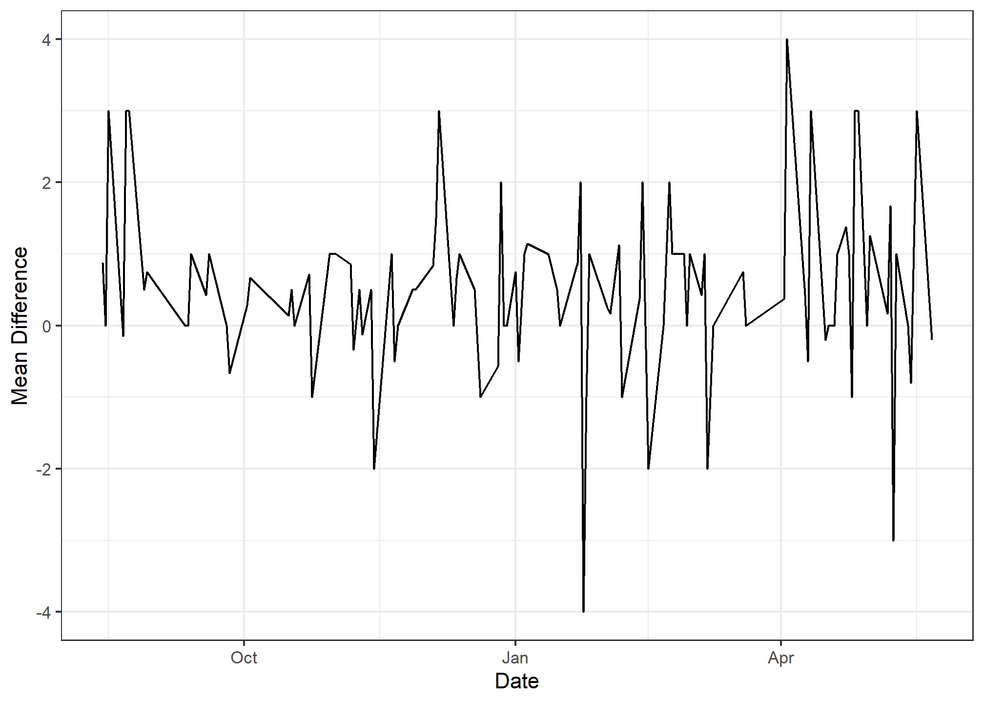
Exercise:

Find the league_id for the England Premier League
Extract all matches for the England Premier League for each day in the "2010/2011" season into a new data set.
Calculate the mean of the difference between home team goals and away team goals for each day in the season.
- You’ll need to separate date and time.
- You’ll also need to use parse_date() before you plot.
Plot this proportion against time.

League <- League_db %>% 
  collect()
  
head(League)

## # A tibble: 6 x 3
##      id country_id name                  
##   <int>      <int> <chr>                 
## 1     1          1 Belgium Jupiler League
## 2  1729       1729 England Premier League
## 3  4769       4769 France Ligue 1        
## 4  7809       7809 Germany 1. Bundesliga 
## 5 10257      10257 Italy Serie A         
## 6 13274      13274 Netherlands Eredivisie

League %>% 
  filter(name =="England Premier League")

## # A tibble: 1 x 3
##      id country_id name                  
##   <int>      <int> <chr>                 
## 1  1729       1729 England Premier League

subMatch <- Match_db %>%
  select(league_id, season, date, home_team_goal, away_team_goal) %>%
  filter(league_id == 1729, season == "2010/2011") %>%
  collect()
  

ave_diff <- subMatch %>%
  separate(col = "date", into = c("date", "time"), sep = " ") %>%
  select(-time) %>%
  group_by(date) %>%
  summarize(mean_diff = mean(home_team_goal - away_team_goal)) %>%
  mutate(date = parse_date(x = date, format = "%Y-%m-%d"))

Your plot should look like this:

ggplot(data = ave_diff, mapping = aes(x = date, y = mean_diff)) +
  geom_line() +
  xlab("Date") +
  ylab("Mean Difference") +
  theme_bw()

You can also visualize your database relationship with the dm package. While the primary and foreign keys are generally recognized, in our case we need to add them manually. You can find more information about the dm package here

install.packages("dm")

library(dm)
dm <- dm_from_src(con, learn_keys = FALSE) %>% 
  dm_add_pk(Country, id) %>%
  dm_add_pk(League, id) %>%
  dm_add_pk(Team, team_api_id) %>%
  dm_add_pk(Team_Attributes, id) %>% 
  dm_add_pk(Match, id) %>%
  dm_add_pk(Player, id) %>%
  dm_add_pk(Player_Attributes, id) %>%
  dm_add_fk(League, country_id, Country) %>%
  dm_add_fk(Match, country_id, Country) %>%
  dm_add_fk(Match, home_team_api_id, Team) %>%
  dm_add_fk(Match, away_team_api_id, Team) %>%
  dm_add_fk(Match, league_id, League) %>% 
  dm_add_fk(Player_Attributes, id, Player) %>%
  dm_add_fk(Team_Attributes, team_fifa_api_id, Team) %>% 
  dm_add_fk(Team_Attributes, team_api_id, Team)

dm %>%
  dm_draw()

Last updated on March 15, 2021

Edit this page

Relational Data and Joins

Learning Outcomes

Relational Data

Example: The Lahman Data Set has Multiple Tables

Each Table has One Purpose: To Describe One Type of Unit

These Tables are Logically Connected

We Define Variables as “Keys” to Identify Rows and to Make Logical Connections Between Tables.

Join Functions in the dplyr Package

Mutating Joins: Inner, Left, Right, Full

inner_join(x, y)

Exercise:

Outer Joins: Left, Right, Full

left_join(x, y)

right_join(x, y)

full_join(x, y)

Exercise:

Duplicate Keys

Filtering Joins Filter Rows in the Left (x) Data Frame:

semi_join(x, y)

anti_join()

Exercise:

Other Key Names

Set operations

Union

intersect

setdiff

Appending Data

References

Appendix on dbplyr

The dbplyr package

Structured Query Language (SQL)

Example using RSQLite with a soccer data set

Setup the Data and Packages

Two Steps to Get Started: Connect and Create Names

Use dplyr to Manipulate the Data

Exercise:

`inner_join(x, y)`

`left_join(x, y)`

`right_join(x, y)`

`full_join(x, y)`

Filtering Joins Filter Rows in the Left (`x`) Data Frame:

`semi_join(x, y)`

`anti_join()`