• Download the in-class written R Markdown here

Projects & RMarkdown

Learning Outcomes:

1. Understand Data Science as context for this course and R in the context of data science.
2. Implement a practical file organization for data science projects.
3. Set the working directory and use relative paths.
4. Install Base R, the RStudio IDE and R Markdown with .
5. Use basic elements of the R language.
6. Use basic elements of R Markdown.
7. Operate within R Studio.

Basic R

Using R as a calculator

The simplest thing you could do with R is to do arithmetic:

1 + 100

## [1] 101

And R will print out the answer, with a preceding “[1].” Don’t worry about this for now. For now think of it as indicating output.

Any time you hit return and the R session shows a “+” instead of a “>,” it means it’s waiting for you to complete the command. If you want to cancel a command you can hit “Esc” and RStudio will give you back the “>” prompt.

When using R as a calculator, the order of operations is the same as you would have learned back in school.

From highest to lowest precedence:

• Parentheses: (, )
• Exponents: ^ or **
• Multiply: *
• Divide: /
• Add: +
• Subtract: -

3 + 5 * 2

## [1] 13

Use parentheses to group operations in order to force the order of evaluation if it differs from the default, or to make clear what you intend.

(3 + 5) * 2

## [1] 16

This can get unwieldy when not needed, but clarifies your intentions. Remember that others may later read your code.

(3 + (5 * (2 ^ 2))) # hard to read
3 + 5 * 2 ^ 2       # clear, if you remember the rules
3 + 5 * (2 ^ 2)     # if you forget some rules, this might help

The text after each line of code is called a “comment.” Anything that follows after the hash (or octothorpe) symbol # is ignored by R when it executes code.

Basic RStudio

Layout

Basic layout

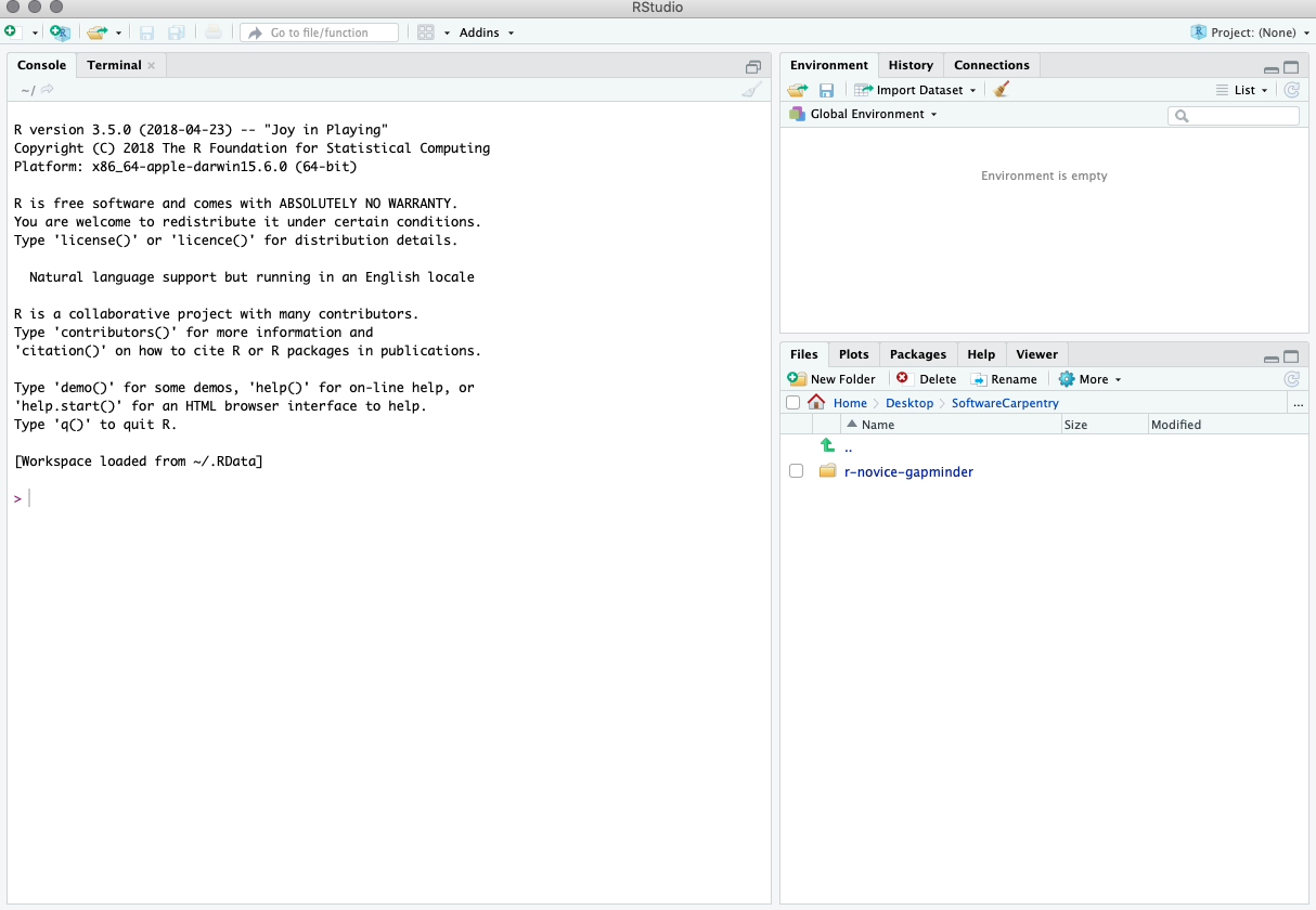
When you first open RStudio, you will be greeted by three panels:

• The interactive R console/Terminal (entire left)
• Environment/History/Connections (tabbed in upper right)
• Files/Plots/Packages/Help/Viewer (tabbed in lower right)

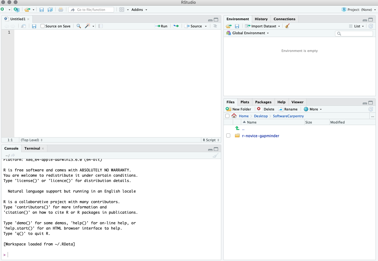
Once you open files, such as R scripts, an editor panel will also open in the top left.

Work flow within RStudio

There are two main ways one can work within RStudio:

1. Test and play within the interactive R console then copy code into a .R file to run later.
   • This works well when doing small tests and initially starting off.
   • It quickly becomes laborious
2. Start writing in a .R file and use RStudio’s short cut keys for the Run command to push the current line, selected lines or modified lines to the interactive R console.
   • This is a great way to start; all your code is saved for later
   • You will be able to run the file you create from within RStudio or using R’s source() function.

Introduction to R

Much of your time in R will be spent in the R interactive console. This is where you will run all of your code, and can be a useful environment to try out ideas before adding them to an R script file. This console in RStudio is the same as the one you would get if you typed in R in your command-line environment.

The first thing you will see in the R interactive session is a bunch of information, followed by a “>” and a blinking cursor. In many ways this is similar to the shell environment you learned about during the shell lessons: it operates on the same idea of a “Read, evaluate, print loop”: you type in commands, R tries to execute them, and then returns a result.

R projects

Working Directory

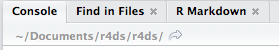
R has a powerful notion of the working directory. This is where R looks for files that you ask it to load, and where it will put any files that you ask it to save. RStudio shows your current working directory at the top of the console:

Or you can prin t it out using

getwd()

## [1] "C:/Users/ckgon/Documents/R/AU-STAT412-612/content/material"

Directories are messy and you should never manually set your working director in an rscript because you may move the directory or someone else may need to open your file.

R experts keep all the files associated with a project together — input data, R scripts, analytical results, figures. This is such a wise and common practice that RStudio has built-in support for this via projects.

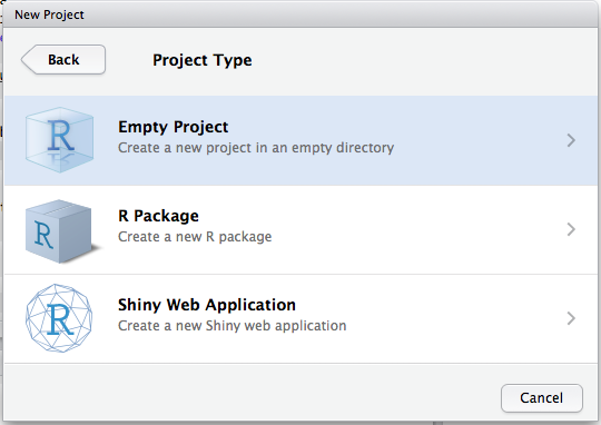
Let’s make a project for you to use while you’re working through the rest of this book. Click File > New Project, then:

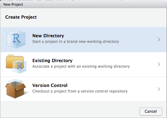
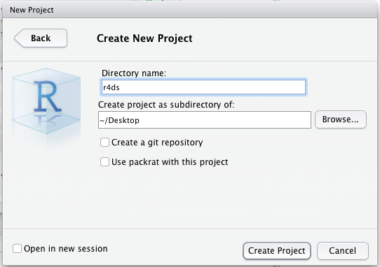Call your project STAT412 or something similar and think carefully about which subdirectory you put the project in. If you don’t store it somewhere sensible, it will be hard to find it in the future!

Once this process is complete, you’ll get a new RStudio project just for this course. Check that the “home” directory of your project is the current working directory:

getwd()
#> [1] C:/Users/kelseygonzalez/Documents/R/AU-STAT412-612

R Markdown

Now, we’ll open up a place to write code. There are two main options for this, scripts and Rmarkdown. Scripts are build just for R code and everything will be evaluated. If you don’t want

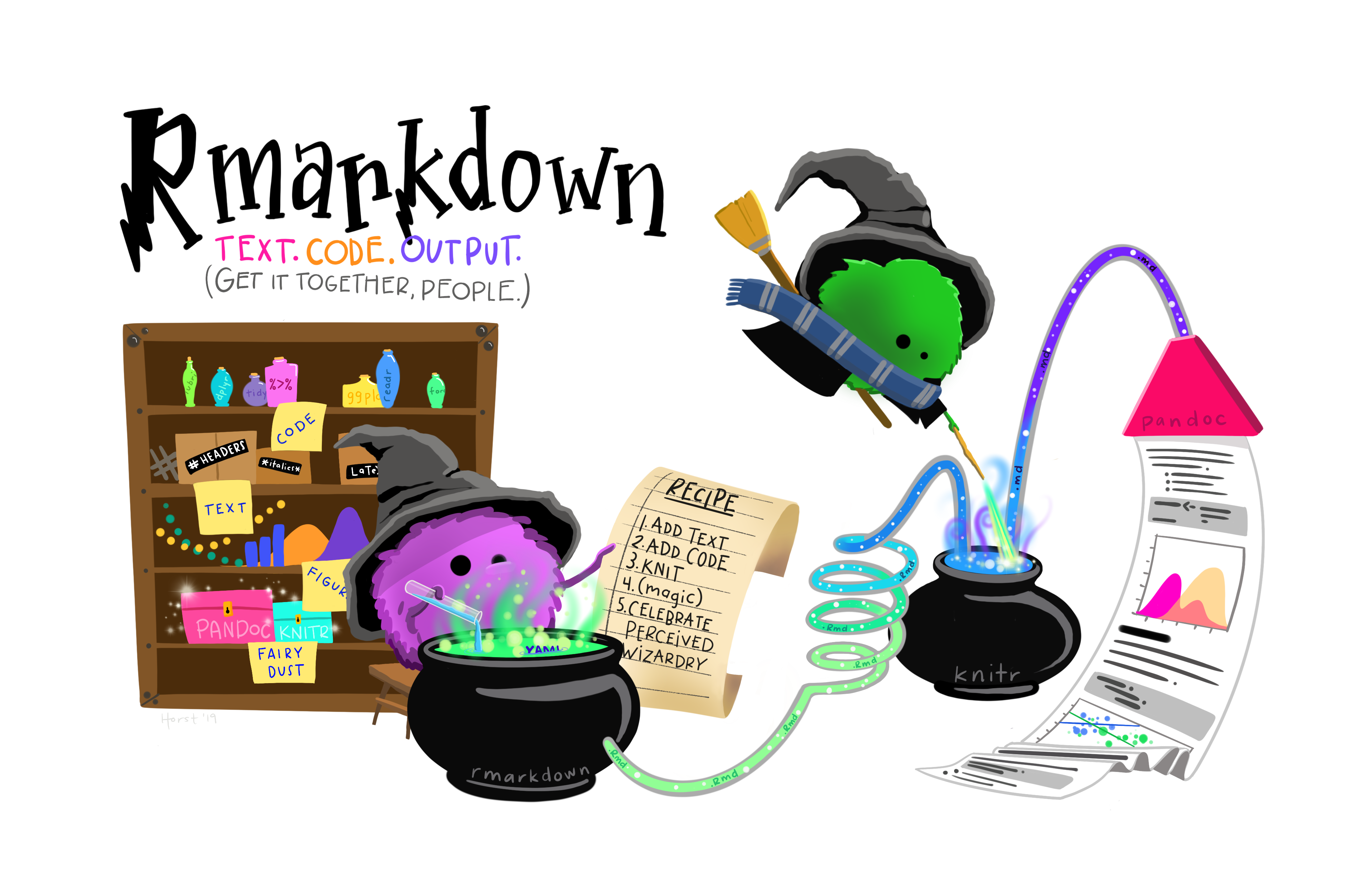
Rmarkdown provides an unified authoring framework for data science, combining your code, its results, and your prose commentary. R Markdown documents are fully reproducible and support dozens of output formats, like PDFs, Word files, slideshows, and more.

R Markdown files are designed to be used in three ways:

1. For communicating to decision makers, who want to focus on the conclusions, not the code behind the analysis.
2. For collaborating with other data scientists (including future you!), who are interested in both your conclusions, and how you reached them (i.e. the code).
3. As an environment in which to do data science, as a modern day lab notebook where you can capture not only what you did, but also what you were thinking.

The key R package is knitr. It allows you to create a document that is a mixture of text and chunks of code. When the document is processed by knitr, chunks of code will be executed, and graphs or other results inserted into the final document.

install.packages("knitr")

Basic Setup

To make these reports, which are ultimately output in HTML, PDF, or Word format, we use a text format called R Markdown. The concept is to use pure text to indicate formatting like bold, italics, and ^superscripts, and to combine this formatting with code that can be executed and output displayed. More on how we do that later. For now, let’s start by creating a new R Markdown file via File > New File > R Markdown… You should then be prompted with a window like:

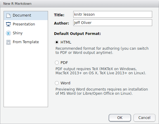
For the title, enter “Class 2-test” and add your name to the author field. Leave the default output format as HTML.

YAML

At the top of the file is the header section, which includes basic information about your document. The heading section is called a YAML (a recursive acronym for “YAML Ain’t Markup Language”). The only field that is absolutely required is the output field, but it is best to include the title, author, and date information, too. Note that immediately below this header is a chunk of code:

```{r setup, include=FALSE}
knitr::opts_chunk$set(echo = TRUE)
```

Followed by text:

## R Markdown
This is an R Markdown document. Markdown is a simple formatting syntax for authoring HTML, 
PDF, and MS Word documents. For more details on using R Markdown see <http://rmarkdown.rstudio.com>.

We will start with formatting in R Markdown syntax, followed by how to include R code in your document.

To try out these formatting examples, start by deleting everything after the header section, so your document only includes:

---
title: "Class 2"
author: "Your Name"
date: "Jan 25, 2021"
output: html_document
---

Basic markdown

Below the header, add this text to your file:

# Introduction to knitr
This is my first knitr document.
Bulleted lists
+ Regular font
+ **bold font**
+ _italic font_
Numbered lists
1. one
2. two
2. three

And the output file is created when we press the Knit button in the top-left part of the screen (or by pressing Shift-Ctrl-K):

Class 2

Your Name

Jan 25, 2021

Introduction to knitr

This is my first knitr document.

Bulleted lists

• Regular font
• bold font
• italic font

Numbered lists

1. one
2. two
3. three

Notice the large font of “Introduction to knitr.” Because we used a single pound sign (#) at the start of the line, this text is formated as a level 1 header. To format lower headers, we add pound signs:

# header 1
## header 2
### header 3
#### header 4

Which are rendered as:

header 1

header 2

header 3

header 4

Links

We can also add hyperlinks to our document, using this syntax: [text we want to link](url address). So to create a link to the American University homepage, we write [American University](https://www.american.edu/). When we run Knit, this is displayed in our document as American University.

Images

Images are also supported, whether they are local files or images on the web. The syntax is almost identical to that for hyperlinks, but in the case of images, we prefix the statement with an exclamation point (!): ![Caption for image](filename)

Here I use an image that I downloaded from Wikimedia into the folder “images” and include a caption:

![The white rhinoceros (_Ceratotherium simum_) (photo by Rob
Hooft)](images/640px-Rhinoceros_male_2003.jpg)

Subscripts and superscripts

Subscripts and superscripts are also supported by wrapping the font in tildes (~) and carets (^), respectively:

Subscript: log~10~
Superscript: r^2^

Subscript: log₁₀ Superscript: r²

Now what happened there? Why aren’t those two on separate lines? When the R Markdown file is interpreted, it assumes adjascent lines should all be part of the same paragraph, unless you indicate otherwise. The way we do this is by adding two blank spaces at the end of a line to indicate a paragraph break:

Subscript: log~10~  <!-- Two spaces at end of line -->
Superscript: r^2^

Subscript: log₁₀
Superscript: r²

Chunks

Now, let’s add in some R code! The best part of knitr is the ability to include code and the output of that code. To do this, we need to add a code chunk.

There are three ways to insert chunks:

• Press ⌘⌥I on macOS or control + alt + I on Windows

• Click on the “Insert” button at the top of the editor window

  

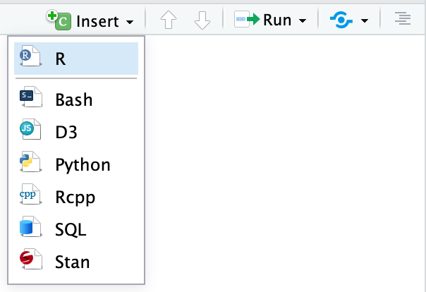
• Manually type all the backticks and curly braces (don’t do this)

You can add names to chunks to make it easier to navigate your document. If you click on the little dropdown menu at the bottom of your editor in RStudio, you can see a table of contents that shows all the headings and chunks. If you name chunks, they’ll appear in the list. If you don’t include a name, the chunk will still show up, but you won’t know what it does.

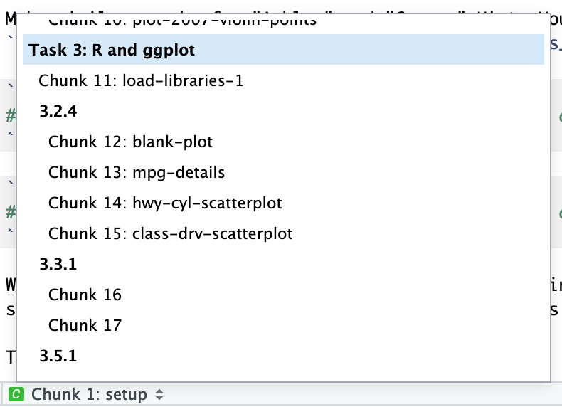
To add a name, include it immediately after the {r in the first line of the chunk. Names cannot contain spaces, but they can contain underscores and dashes. All chunk names in your document must be unique.

Basic R Continued

Mathematical functions

R has many built in mathematical functions. To call a function, we can type its name, followed by open and closing parentheses. Anything we type inside the parentheses is called the function’s arguments:

sin(1)  # trigonometry functions

## [1] 0.841471

log(1)  # natural logarithm

## [1] 0

log10(10) # base-10 logarithm

## [1] 1

exp(0.5) # e^(1/2)

## [1] 1.648721

How do I remember these functions?

Don’t worry about trying to remember every function in R. You can look them up on Google, or if you can remember the start of the function’s name, use the tab completion in RStudio.

This is one advantage that RStudio has over R on its own, it has auto-completion abilities that allow you to more easily look up functions, their arguments, and the values that they take.

Typing a ? before the name of a command will open the help page for that command. When using RStudio, this will open the ‘Help’ pane; if using R in the terminal, the help page will open in your browser. The help page will include a detailed description of the command and how it works. Scrolling to the bottom of the help page will usually show a collection of code examples which illustrate command usage. We’ll go through an example later.

Comparing things

We can also do comparisons in R:

1 == 1  # equality (note two equals signs, read as "is equal to")

## [1] TRUE

1 != 2  # inequality (read as "is not equal to")

## [1] TRUE

1 < 2  # less than

## [1] TRUE

1 <= 1  # less than or equal to

## [1] TRUE

1 > 0  # greater than

## [1] TRUE

1 >= -9 # greater than or equal to

## [1] TRUE

Variables and assignment

We can store values in variables using the assignment operator <-, like this:

x <- 1/40

Notice that assignment does not print a value. Instead, we stored it for later in something called a variable. x now contains the value 0.025:

x

## [1] 0.025

Look for the Environment tab in the top right panel of RStudio, and you will see that x and its value have appeared. Our variable x can be used in place of a number in any calculation that expects a number:

log(x)

## [1] -3.688879

Notice also that variables can be reassigned:

x <- 100

x used to contain the value 0.025 and now it has the value 100.

Assignment values can contain the variable being assigned to:

x <- x + 1 #notice how RStudio updates its description of x on the top right tab
y <- x * 2

The right hand side of the assignment can be any valid R expression. The right hand side is fully evaluated before the assignment occurs.

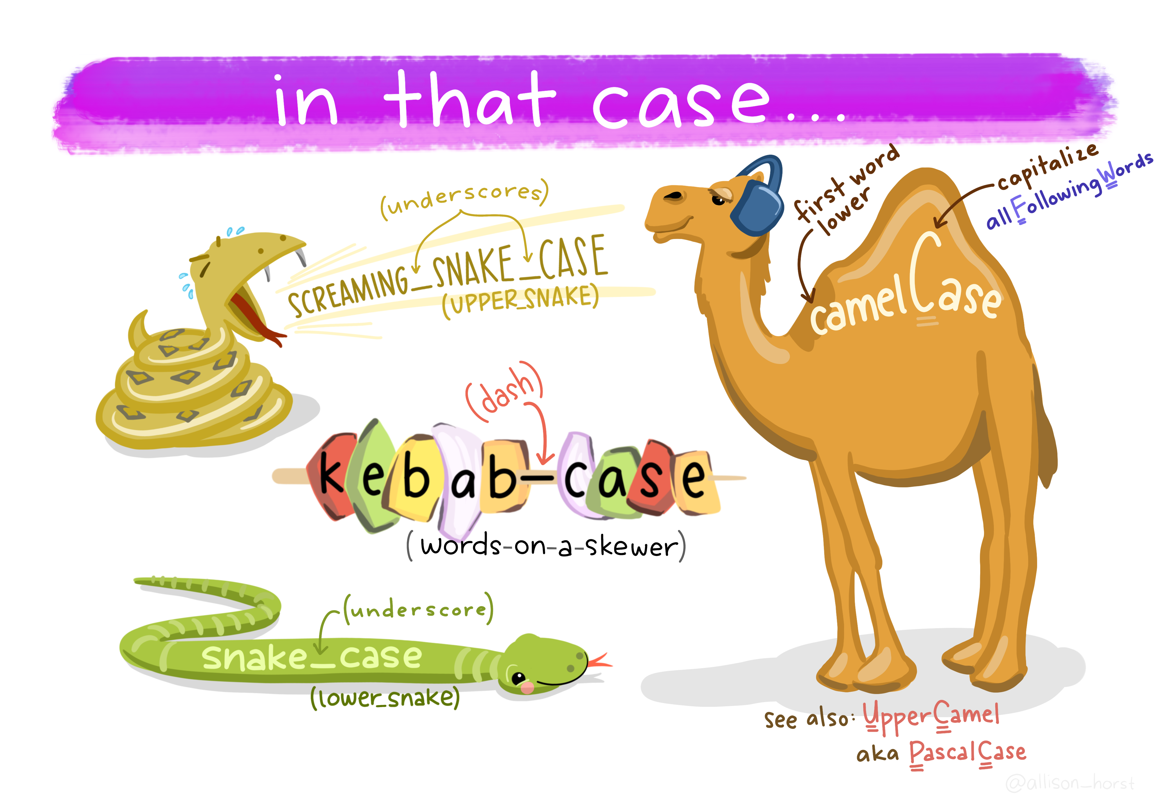
Variable names can contain letters, numbers, underscores and periods but no spaces. They must start with a letter or a period followed by a letter (they cannot start with a number nor an underscore). Variables begining with a period are hidden variables. Different people use different conventions for long variable names, these include

• periods.between.words
• underscores_between_words
• camelCaseToSeparateWords

What you use is up to you, but be consistent.

R Markdown chunk options

There’s a lot we can do to control what actually prints out to our knitted document. If we just want to display the output but not the code itself, we can add echo = FALSE to indicate that.

You can also control code chunks in a number of other ways:

• eval = FALSE to show code but not to execute it
• results = "hide" to suppress any results from being included in output
• warning = FALSE and message = FALSE to suppress warnings and messages, respectively, from being shown

Let’s test this out:

```{r echo = FALSE}
x <- 5
y <- 3
```

Even though we set echo = FALSE, the code is still executed and we can reference products of that code through in-line code chunks. In this case, we want to reference the value stored in our r.squared variable in our document text. We use in-line code to do so. In-line code is wrapped in single backticks (`) and we skip the braces, as opposed to triple backticks and braces we used for separate code blocks. So we can write: `r x * y` in-text for it to evaluate like this:

x times y is 15

You can find more about options under resources

Some simple data

Let’s get some data loaded so we can do some very simple exploration of a dataset. The mtcars dataset comes pre-loaded with R, and although it’s boring, it will serve our purposes!

data(mtcars)

Let’s try out a few commands we can use to explore our data.

mtcars
nrow(mtcars)
ncol(mtcars)
dim(mtcars)
head(mtcars)
tail(mtcars)
View(mtcars)
summary(mtcars)

What do these do?

References

Wickham and Grolemund. 2016. R for data science O’Reilly Media, Inc. 

• Chapter 8: Projects
• Chapter 27: R Markdown
• Producing Reports With knitr

Additional resources

• Knitr in a knutshell tutorial
• Dynamic Documents with R and knitr (book)
• An awesome cookbook of R Markdown solutions
• R Markdown documentation
• R Markdown cheat sheet
• An awesome cookbook of R Markdown solutions
• Getting started with R Markdown
• R Markdown: The Definitive Guide (book by Rstudio team)
• Reproducible Reporting
• The Ecosystem of R Markdown
• Guide to writing bibliography sections in R Markdown documents
• Creating Word templates to apply to knitr documents