Data Wrangling with `dplyr`
- Download the in-class written R Markdown here.
Introduction
- Real world data is always messy to start
- Variables may be missing
- Values may be missing
- There can be duplicate rows
- Variables may have different names in different tables for the same attribute
- Numbers can be stored as characters
- The data may be structured for ease of human input rather than analysis
- Unsorted or sorted in a different order than we want
- The tidyverse
dplyrpackage provides tools to speed up the manipulation of data- Uses data frames to create consistent structure
- Uses the forward pipe operator,
%>%, to facilitate transparency/readability - Compared to the predecessor
plyrlibrary,dplyris 20X - 100X faster - Enables faster Exploratory Data Analysis (EDA) with
ggplot2
Learning Outcomes
- Describe data frames in R and tidyverse tibbles
- Use basic functions of dplyr to manipulate single data frames/tibbles by rows, by columns (variables), and by groups
- Choose rows by column (variable) values
filter() - Arrange (sort) rows by column (variable) values:
arrange() - Choose columns (variables) by names
select() - Rename columns (variables):
rename() - Add/modify new/existing columns (variables):
mutate()ortransmute() - Group rows by columns (variables):
group_by() - Calculate summary statistics of Columns with or without grouping.
summarize(),group_by()
- Choose rows by column (variable) values
Introduction to the dplyrpackage
Background on Data Frames and Tibbles
-
The R language uses two kinds of vectors to manage data: Atomic Vectors and Lists
- Atomic vectors are sequences of elements of the same data type.
- Lists are data structures where the elements do Not have to be the same type
-
Vectors have two main attributes: Length and data Type
-
R has six data types:
- logical,
- integer,
- double,
- character,
- complex, and
- raw(byte-level data).
-
Integer and double vectors are collectively known as numeric vectors
Data Frames
- A data frame in R is a special kind of list: a data.frame object
- Every element in a data.frame is an atomic vector with the same length
- This means data frames are rectangular matrices of columns and rows.
- The columns can be of different types
- The elements within each column must be the same type
- Each column has the same number of rows
- Some rows may be missing the value for a given column. They should have
NAin the row for that column.
- Consider a set of data about a number of observational or experimental units
- In
mpgthe cars were the observational units - the things on which someone collected data.
- In
- The data set includes information on different attributes or characteristics of the units.
- These attributes are called the variables as their values can change from unit to unit.
- These variables are the columns of the data frame.
- In
mpgthese are: - manufacturer, model, displ, year, cyl, trans, drv, cty, hwy, fl, class
- In
- The observed values for each of the attributes are the rows.
- for
mpgthe first row of observations are: - audi, a4, 1.8, 1999, 4, auto(l5), f, 18, 29, p, compact
- for
- For example, in the
msleepdata frame, the observations are animals and the the variables are properties of those animals (body weight, total sleep time, etc). - You can create data frames using the
data.frame()oras.data.frame()
Tibbles
-
Tibbles are a tidyverse version of an R data.frame class of object.
-
They have all the same features as a regular R data frame with a few nicer attributes, e.g., for printing.
-
You can create tibbles with the functions
tibble::tibble()oras.tibble() -
You can create small tibbles with
tibble::tribble() -
Since we were are focused on the tidyverse, we will use the terms data frame and tibble as synonyms for each other in general usage.
-
Data frames/tibbles are the fundamental data type in most analyses.
-
Many people work with data in table-like structures such as data frames
- A data frame is similar to a “Named Range” on an Excel worksheet where the first row contains the variable names
- A data frame is similar to a database table
The dplyr Package
- The dplyr package is a tidyverse package
- It is installed and loaded with the tidyverse package and can be installed/loaded on its own as well.
- The dplyr package is designed to enable users to manipulate or transform data in data frames/tibbles.
- To goal is to support users by using a consistent “grammar of data,” leading to faster and more reliable results.
- dplyr’s functions have names similar to those in other data manipulation tools or languages, e.g., SQL (Structured QUery Language), so it is easier to learn and apply.
dplyr Functions Support Common Manipulations/Transformations/Operations on Data and Data Frames
- Common operations on a data frame during an analysis include:
- Select specific variables:
select() - Choose specific observational units based on the values of their attributes:
filter() - Create new variables or modify existing variables:
mutate() - Reorder the observational units:
arrange() - Create summary statistics from many observational units:
summarize() - Group the observational units by the values of some variables:
group_by()
- Select specific variables:
- Think of the dplyr functions (like other functions) as “verbs” that do things with the data.
- We can characterize them base on the component of the data set they work with: (bold are the most commonly used)
- Rows:
filter()chooses rows based on column values.arrange()changes the order of the rows.
- Columns:
select()changes whether or not a column is included.rename()changes the name of columns.mutate()changes the values of columns and creates new columns.relocate()changes the order of the columns.
- Groups of rows:
summarize()collapses a group into a single row.
- These are all “Single Table” verbs meaning they operate on a single data frame.
- There are more dplyr functions (verbs) as well
- Next week in dplyr Part 2 we will address additional functions (verbs) for working across rows and columns
- Later on in the course we will address dplyr verbs for reshaping data frames and working with two data frames at once. # Getting started with penguins Let’s explore our data first. We’ll be using the penguins dataset again, this time specifically to see how we can wrangle this data into new forms.
# install.packages("palmerpenguins")
library(tidyverse)
library(palmerpenguins)
data("penguins")

What I imagine it looked like when the penguins were weighed:
Never get bored of penguins getting weighed.. from r/aww
We have a few options to preview our dataframe that we’ve discussed before. However, now that we have the tidyverse loaded, we can rely on my favorite, glimpse()
glimpse(penguins)
## Rows: 344
## Columns: 8
## $ species [3m[90m<fct>[39m[23m Adelie, Adelie, Adelie, Adelie, Adelie, Adelie, A...
## $ island [3m[90m<fct>[39m[23m Torgersen, Torgersen, Torgersen, Torgersen, Torge...
## $ bill_length_mm [3m[90m<dbl>[39m[23m 39.1, 39.5, 40.3, NA, 36.7, 39.3, 38.9, 39.2, 34....
## $ bill_depth_mm [3m[90m<dbl>[39m[23m 18.7, 17.4, 18.0, NA, 19.3, 20.6, 17.8, 19.6, 18....
## $ flipper_length_mm [3m[90m<int>[39m[23m 181, 186, 195, NA, 193, 190, 181, 195, 193, 190, ...
## $ body_mass_g [3m[90m<int>[39m[23m 3750, 3800, 3250, NA, 3450, 3650, 3625, 4675, 347...
## $ sex [3m[90m<fct>[39m[23m male, female, female, NA, female, male, female, m...
## $ year [3m[90m<int>[39m[23m 2007, 2007, 2007, 2007, 2007, 2007, 2007, 2007, 2...
It looks like there are 7 variables or columns that we have to work with.
species: penguin species (Chinstrap, Adélie, or Gentoo)bill_length_mm: bill length (mm)bill_depth_mm: bill depth (mm)flipper_length_mm: flipper length (mm)body_mass_g: body mass (g)island: island name (Dream, Torgersen, or Biscoe) in the Palmer Archipelago (Antarctica)sex: penguin sex
Selecting columns
To select columns of a data frame, use select(). The select() function extracts (subsets) variables (columns) and place them into a new smaller (temporary) data frame. The first argument to this function is the data frame (penguins), and the subsequent arguments are the columns to keep.
select(penguins, species, body_mass_g, sex)
# Select specific variables by their names
select(penguins, species, body_mass_g)

# Select a range of contiguous (adjacent or sequential) variables with `:`
select(penguins, species:bill_length_mm)

# Select all variables **except certain ones** with `-`, the minus sign
select(penguins, -year, -island)

# Select all variables **except within a contiguous range of columns**.

select(penguins, -(species:island))
Helper Functions for select()
-
THere are several “helper functions” you can use as arguments inside
select()- These helper functions are actually part of the tidyselect package that is always installed and loaded with dplyr
- See help for “language” from tidyselect or help on “starts_with” from tidyselect
-
These helper functions reduce the need to specify each and every variable you want or don’t want.
- Some data frames may have 1000s of variables in them
-
Variables names in a data frame are always character strings so the helper functions compare the variable names to the character patterns you provide.
-
starts_with("abc"): matches names that begin with"abc".
select(penguins, starts_with("bill"))
## # A tibble: 344 x 2
##    bill_length_mm bill_depth_mm
##             <dbl>         <dbl>
##  1           39.1          18.7
##  2           39.5          17.4
##  3           40.3          18
##  4           NA            NA
##  5           36.7          19.3
##  6           39.3          20.6
##  7           38.9          17.8
##  8           39.2          19.6
##  9           34.1          18.1
## 10           42            20.2
## # ... with 334 more rows
ends_with("xyz"): matches names that end with"xyz".
select(penguins, ends_with("mm"))
## # A tibble: 344 x 3
##    bill_length_mm bill_depth_mm flipper_length_mm
##             <dbl>         <dbl>             <int>
##  1           39.1          18.7               181
##  2           39.5          17.4               186
##  3           40.3          18                 195
##  4           NA            NA                  NA
##  5           36.7          19.3               193
##  6           39.3          20.6               190
##  7           38.9          17.8               181
##  8           39.2          19.6               195
##  9           34.1          18.1               193
## 10           42            20.2               190
## # ... with 334 more rows
contains("ijk"): matches names that contain"ijk".
select(penguins, contains("length"), species)
## # A tibble: 344 x 3
##    bill_length_mm flipper_length_mm species
##             <dbl>             <int> <fct>
##  1           39.1               181 Adelie
##  2           39.5               186 Adelie
##  3           40.3               195 Adelie
##  4           NA                  NA Adelie
##  5           36.7               193 Adelie
##  6           39.3               190 Adelie
##  7           38.9               181 Adelie
##  8           39.2               195 Adelie
##  9           34.1               193 Adelie
## 10           42                 190 Adelie
## # ... with 334 more rows
matches("(.)\\1"): selects variables that match a regular expression (REGEX).- This one matches any variables with two repeated characters, e.g., “YY.”
- You’ll learn more about regular expressions in the class on strings and stringr.
num_range("x", 1:3): matchesx1,x2, andx3for whatever numerical sequence you provide- This can be useful for data sets with variables such as month1, month2, month3 …, or FY18, FY19, FY20, ….
Filtering rows
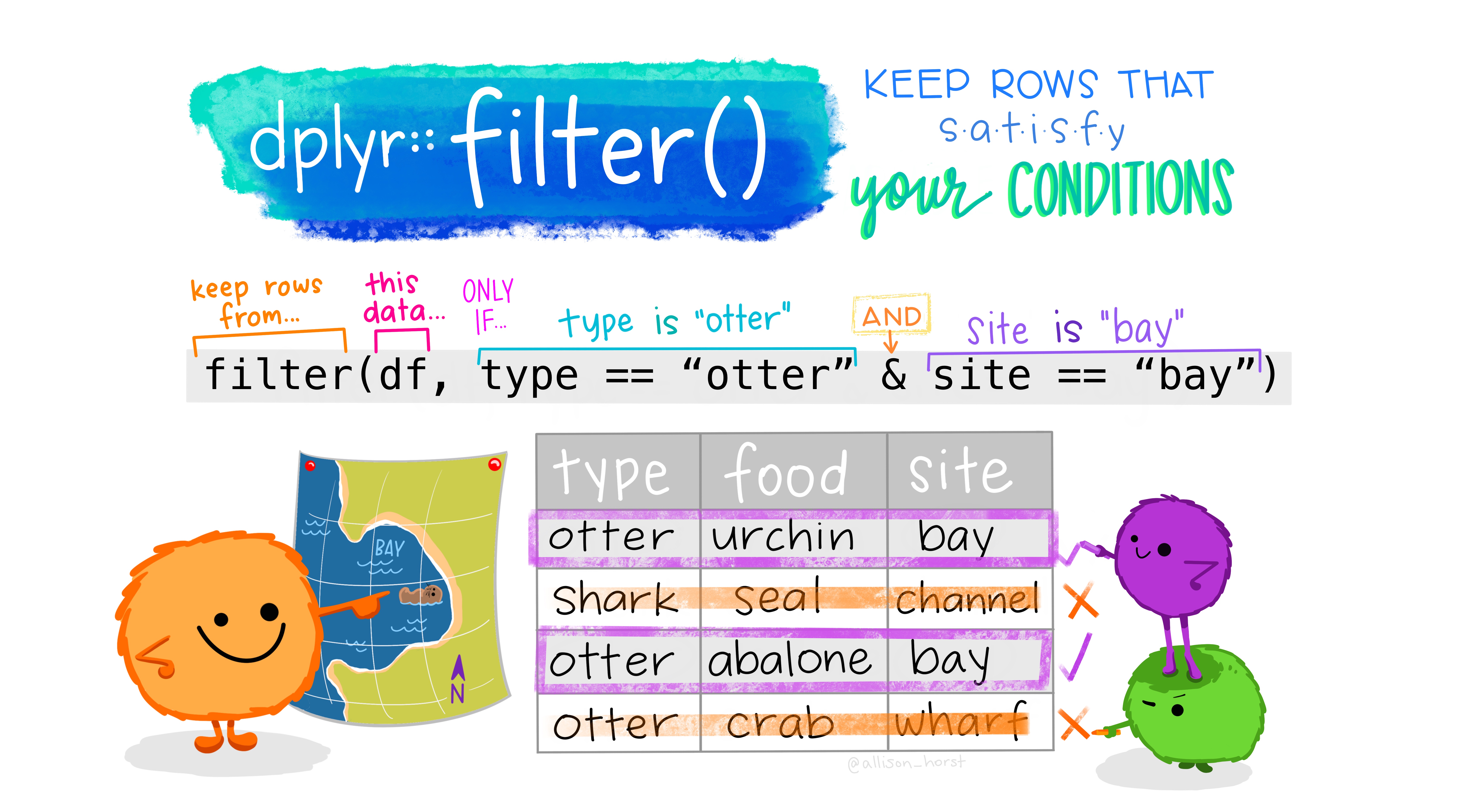
Choose Rows Based on Values of Certain Variables
-
The dplyr
filter()function allows us to choose (subset/extract) only certain rows (observations) based on the values of the variables in those rows. -
We create conditions and
filter()selects the rows satisfying these conditions (returnTRUE).- We can use logical comparisons, and use AND (
&) or OR (|) as well
- We can use logical comparisons, and use AND (
-
Let’s extract all the penguins from New York that occurred in January or the 1st month of the year.
filter(penguins, island == "Biscoe")
filter(penguins, year <= "2008")
The filter function works with most boolean operators, namely:
| Operator | Description |
|---|---|
< |
less than |
<= |
less than or equal to |
> |
greater than |
>= |
greater than or equal to |
== |
exactly equal to |
!= |
not equal to |
!x |
Not x |
x | y |
x OR y |
x & y |
x AND y |
isTRUE(x) |
test if X is TRUE |
Multiple Conditions
- Graphical depiction of logical operations:
- Blue is TRUE (to be included) and White is FALSE (not included)
!means Not (!TRUE means FALSE)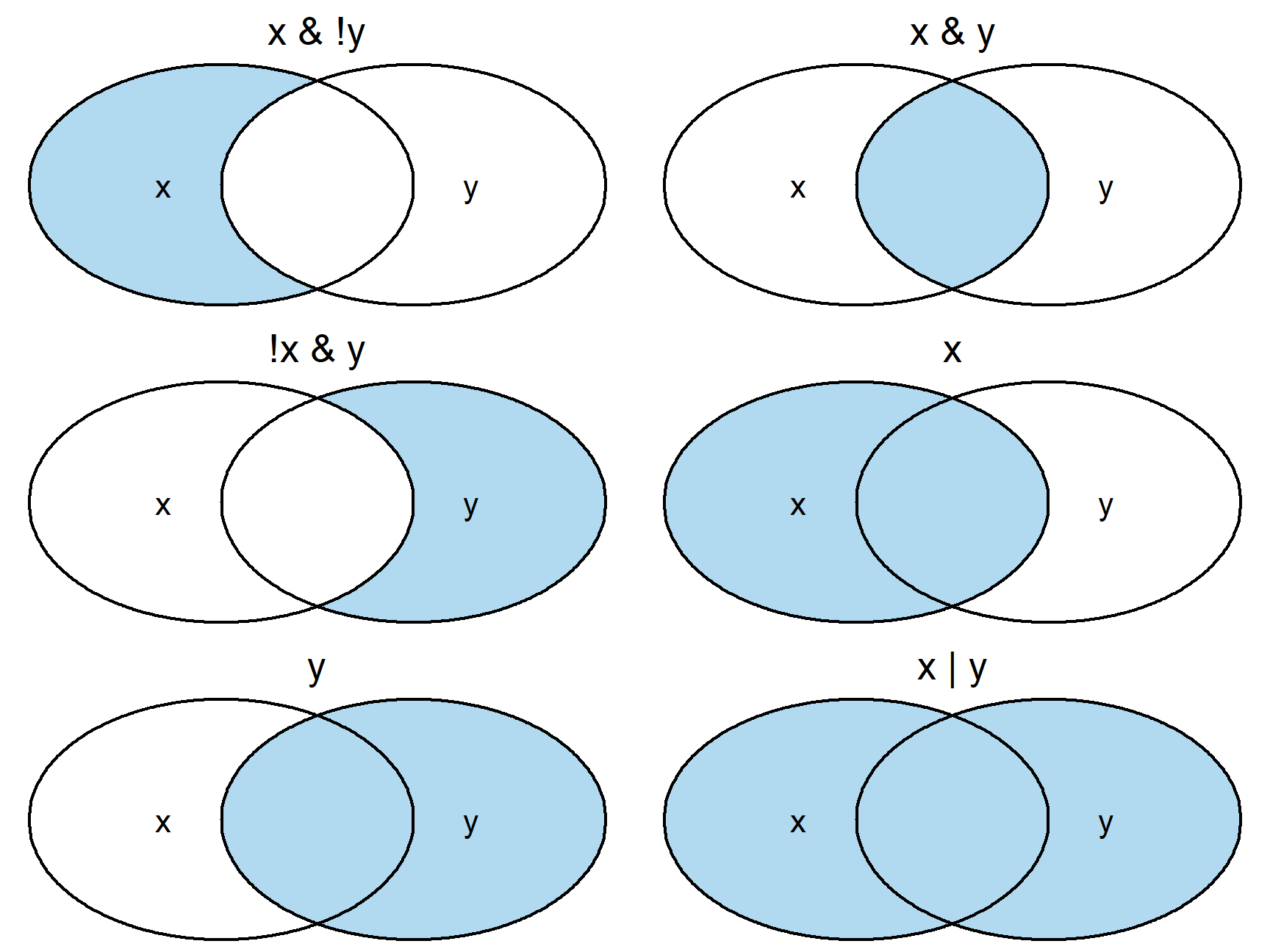
and
-
Example: Let’s get all penguins from Biscoe island and Gentoo species.
-
The And operator is the most commonly used. So, if you just separate the logical conditions by a comma,
filter()will perform the And operation by default .
filter(penguins, island == "Biscoe", origin == "Gentoo")
-
If you don’t know the possible values of a categorical variable, you have two options:
- If the variable is a factor, use
levels() - Otherwise, use
unique()
- If the variable is a factor, use
levels(penguins$species)
## [1] "Adelie" "Chinstrap" "Gentoo"
count(penguins, species)
## # A tibble: 3 x 2
##   species       n
## * <fct>     <int>
## 1 Adelie      152
## 2 Chinstrap    68
## 3 Gentoo      124
or
# using the or | operator

filter(penguins, species == "Chinstrap" | species == "Gentoo")
## # A tibble: 192 x 8
##    species island bill_length_mm bill_depth_mm flipper_length_~ body_mass_g
##    <fct>   <fct>           <dbl>         <dbl>            <int>       <int>
##  1 Gentoo  Biscoe           46.1          13.2              211        4500
##  2 Gentoo  Biscoe           50            16.3              230        5700
##  3 Gentoo  Biscoe           48.7          14.1              210        4450
##  4 Gentoo  Biscoe           50            15.2              218        5700
##  5 Gentoo  Biscoe           47.6          14.5              215        5400
##  6 Gentoo  Biscoe           46.5          13.5              210        4550
##  7 Gentoo  Biscoe           45.4          14.6              211        4800
##  8 Gentoo  Biscoe           46.7          15.3              219        5200
##  9 Gentoo  Biscoe           43.3          13.4              209        4400
## 10 Gentoo  Biscoe           46.8          15.4              215        5150
## # ... with 182 more rows, and 2 more variables: sex <fct>, year <int>
# Second way: using the %in% operator
filter(penguins, species %in% c("Chinstrap", "Gentoo"))
## # A tibble: 192 x 8
##    species island bill_length_mm bill_depth_mm flipper_length_~ body_mass_g
##    <fct>   <fct>           <dbl>         <dbl>            <int>       <int>
##  1 Gentoo  Biscoe           46.1          13.2              211        4500
##  2 Gentoo  Biscoe           50            16.3              230        5700
##  3 Gentoo  Biscoe           48.7          14.1              210        4450
##  4 Gentoo  Biscoe           50            15.2              218        5700
##  5 Gentoo  Biscoe           47.6          14.5              215        5400
##  6 Gentoo  Biscoe           46.5          13.5              210        4550
##  7 Gentoo  Biscoe           45.4          14.6              211        4800
##  8 Gentoo  Biscoe           46.7          15.3              219        5200
##  9 Gentoo  Biscoe           43.3          13.4              209        4400
## 10 Gentoo  Biscoe           46.8          15.4              215        5150
## # ... with 182 more rows, and 2 more variables: sex <fct>, year <int>
-
You should still know the logical operators in case the filtering gets complicated.
-
Let’s extract the Biscoe Gentoo penguins and the Dream Adelie penguins.
filter(penguins,
       (island == "Biscoe" & species == "Gentoo") |
         (island == "Dream" & species == "Adelie"))
Missing Values
- if you explicitly want to extract missing values, we have to use
is.na(x)instead ofx == NA.
filter(penguins, is.na(sex))
## # A tibble: 11 x 8
##    species island bill_length_mm bill_depth_mm flipper_length_~ body_mass_g
##    <fct>   <fct>           <dbl>         <dbl>            <int>       <int>
##  1 Adelie  Torge~           NA            NA                 NA          NA
##  2 Adelie  Torge~           34.1          18.1              193        3475
##  3 Adelie  Torge~           42            20.2              190        4250
##  4 Adelie  Torge~           37.8          17.1              186        3300
##  5 Adelie  Torge~           37.8          17.3              180        3700
##  6 Adelie  Dream            37.5          18.9              179        2975
##  7 Gentoo  Biscoe           44.5          14.3              216        4100
##  8 Gentoo  Biscoe           46.2          14.4              214        4650
##  9 Gentoo  Biscoe           47.3          13.8              216        4725
## 10 Gentoo  Biscoe           44.5          15.7              217        4875
## 11 Gentoo  Biscoe           NA            NA                 NA          NA
## # ... with 2 more variables: sex <fct>, year <int>
filter(penguins, !is.na(sex))
## # A tibble: 333 x 8
##    species island bill_length_mm bill_depth_mm flipper_length_~ body_mass_g
##    <fct>   <fct>           <dbl>         <dbl>            <int>       <int>
##  1 Adelie  Torge~           39.1          18.7              181        3750
##  2 Adelie  Torge~           39.5          17.4              186        3800
##  3 Adelie  Torge~           40.3          18                195        3250
##  4 Adelie  Torge~           36.7          19.3              193        3450
##  5 Adelie  Torge~           39.3          20.6              190        3650
##  6 Adelie  Torge~           38.9          17.8              181        3625
##  7 Adelie  Torge~           39.2          19.6              195        4675
##  8 Adelie  Torge~           41.1          17.6              182        3200
##  9 Adelie  Torge~           38.6          21.2              191        3800
## 10 Adelie  Torge~           34.6          21.1              198        4400
## # ... with 323 more rows, and 2 more variables: sex <fct>, year <int>
Pipes
What if you want to select and filter at the same time? There are three ways to do this: use intermediate steps, nested functions, or pipes.
With intermediate steps, you create a temporary data frame and use that as input to the next function, like this:
penguins_biscoe <- filter(penguins, island == "Biscoe")
penguins_biscoe <- select(penguins_biscoe, species, body_mass_g, sex)
This is readable, but can clutter up your workspace with lots of objects that you have to name individually. With multiple steps, that can be hard to keep track of.
You can also nest functions (i.e. one function inside of another), like this:
penguins_Biscoe <-
  select(
    filter(penguins, island == "Biscoe"),
    species, body_mass_g, sex)
This is handy, but can be difficult to read if too many functions are nested, as R evaluates the expression from the inside out (in this case, filtering, then selecting).
The last option, pipes, are a powerful addition to R. Pipes let you take the output of one function and send it directly to the next, which is useful when you need to do many things to the same dataset. Pipes in R look like %>% and are made available via the magrittr package, installed automatically with dplyr. If you use RStudio, you can type the pipe with Ctrl + Shift + M if you have a PC or Cmd + Shift + M if you have a Mac.
penguins %>%
    filter(island == "Biscoe") %>%
    select(species, body_mass_g, sex)
## # A tibble: 168 x 3
##    species body_mass_g sex
##    <fct>         <int> <fct>
##  1 Adelie         3400 female
##  2 Adelie         3600 male
##  3 Adelie         3800 female
##  4 Adelie         3950 male
##  5 Adelie         3800 male
##  6 Adelie         3800 female
##  7 Adelie         3550 male
##  8 Adelie         3200 female
##  9 Adelie         3150 female
## 10 Adelie         3950 male
## # ... with 158 more rows
In the above code, we use the pipe to send the penguins dataset first through filter() to keep rows where island is “Biscoe,” then through select() to keep only the species, body_mass_g,and sex columns. Since %>% takes the object on its left and passes it as the first argument to the function on its right, we don’t need to explicitly include the data frame as an argument to the filter() and select() functions any more.
Some may find it helpful to read the pipe like the word “then.” For instance, in the above example, we take the data frame penguins, then we filter for rows with island == "Biscoe", then we select columns species, body_mass_g,and sex. The dplyr functions by themselves are somewhat simple, but by combining them into linear workflows with the pipe, we can accomplish more complex manipulations of data frames.
If we want to create a new object with this smaller version of the data, we can assign it a new name:
penguins_biscoe <- penguins %>%
    filter(island == "Biscoe") %>%
    select(species, body_mass_g, sex)

penguins_biscoe
## # A tibble: 168 x 3
##    species body_mass_g sex
##    <fct>         <int> <fct>
##  1 Adelie         3400 female
##  2 Adelie         3600 male
##  3 Adelie         3800 female
##  4 Adelie         3950 male
##  5 Adelie         3800 male
##  6 Adelie         3800 female
##  7 Adelie         3550 male
##  8 Adelie         3200 female
##  9 Adelie         3150 female
## 10 Adelie         3950 male
## # ... with 158 more rows
Note that the final data frame (penguins_biscoe) is the leftmost part of this expression becuase it is receiving an assignment.
Exercise
Using pipes, subset the
penguinsdata to include all species EXCEPT Adelie and retain the species column in addition to those relating to their bill.Solution
penguins %>%
    filter(species != "Adelie") %>%
    select(species, bill_length_mm, bill_depth_mm)
Arrange
Rearrange the Order of the Rows
- Use
arrange()to order rows by the value of one or more variables. - The sort order for character vectors will depend on the collating sequence of the locale in use: see help for
locales().
penguins %>%
  arrange(body_mass_g)
- The default is to arrange in ascending order from top to bottom so the lowest number is on top.
- Use the
desc()function on the variable insidearrange()to arrange in descending order - For numerics you can use
-instead
# body_mass_g is numeric
penguins %>%
  arrange(desc(body_mass_g))
penguins %>%
  arrange(-body_mass_g)

# island is categorical
penguins %>%
  arrange(desc(island))
- If there are ties with one variable, you can break the ties by arranging by another variable.
penguins %>%
  arrange(island, body_mass_g)
## # A tibble: 344 x 8
##    species island bill_length_mm bill_depth_mm flipper_length_~ body_mass_g
##    <fct>   <fct>           <dbl>         <dbl>            <int>       <int>
##  1 Adelie  Biscoe           36.5          16.6              181        2850
##  2 Adelie  Biscoe           36.4          17.1              184        2850
##  3 Adelie  Biscoe           34.5          18.1              187        2900
##  4 Adelie  Biscoe           37.9          18.6              193        2925
##  5 Adelie  Biscoe           37.7          16                183        3075
##  6 Adelie  Biscoe           37.9          18.6              172        3150
##  7 Adelie  Biscoe           35.7          16.9              185        3150
##  8 Adelie  Biscoe           38.1          17                181        3175
##  9 Adelie  Biscoe           40.5          17.9              187        3200
## 10 Adelie  Biscoe           39.7          17.7              193        3200
## # ... with 334 more rows, and 2 more variables: sex <fct>, year <int>
penguins %>%
  arrange(island, desc(body_mass_g))
## # A tibble: 344 x 8
##    species island bill_length_mm bill_depth_mm flipper_length_~ body_mass_g
##    <fct>   <fct>           <dbl>         <dbl>            <int>       <int>
##  1 Gentoo  Biscoe           49.2          15.2              221        6300
##  2 Gentoo  Biscoe           59.6          17                230        6050
##  3 Gentoo  Biscoe           51.1          16.3              220        6000
##  4 Gentoo  Biscoe           48.8          16.2              222        6000
##  5 Gentoo  Biscoe           45.2          16.4              223        5950
##  6 Gentoo  Biscoe           49.8          15.9              229        5950
##  7 Gentoo  Biscoe           48.4          14.6              213        5850
##  8 Gentoo  Biscoe           49.3          15.7              217        5850
##  9 Gentoo  Biscoe           55.1          16                230        5850
## 10 Gentoo  Biscoe           49.5          16.2              229        5800
## # ... with 334 more rows, and 2 more variables: sex <fct>, year <int>
- Observations with missing values are always placed at the end (even when using the
desc()function)
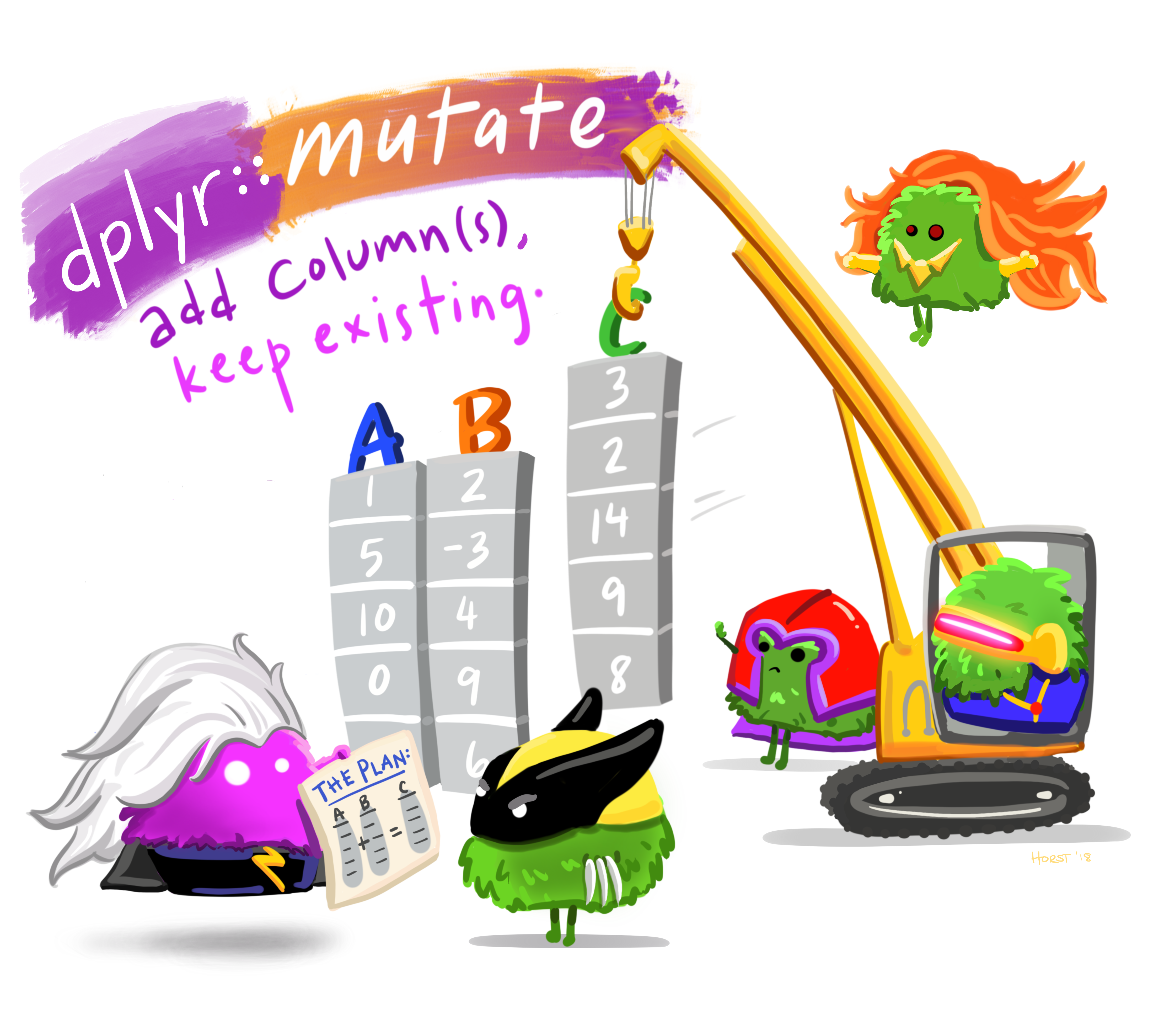
Mutate
- The variables we have are usually not enough for all the questions we want to look at in an analysis.
- We often use a
log()function to transform positive data to reduce skew or try to make associations more linear. - We also like to combine variables to create new attributes based on existing attributes.
- We often use a
Therefore, we may want to create new columns based on the values in existing columns, for example to do unit conversions, or to find the ratio of values in two columns. For this we’ll use mutate().
- We use
mutate()to create new variables from old - adds one or more columns to our temporary data frame. - We will do this a lot!
We might be interested in the flipper length of penguins in cm instead of milimeters:
penguins %>%
    mutate(flipper_length_cm = flipper_length_mm / 10)
## # A tibble: 344 x 9
##    species island bill_length_mm bill_depth_mm flipper_length_~ body_mass_g
##    <fct>   <fct>           <dbl>         <dbl>            <int>       <int>
##  1 Adelie  Torge~           39.1          18.7              181        3750
##  2 Adelie  Torge~           39.5          17.4              186        3800
##  3 Adelie  Torge~           40.3          18                195        3250
##  4 Adelie  Torge~           NA            NA                 NA          NA
##  5 Adelie  Torge~           36.7          19.3              193        3450
##  6 Adelie  Torge~           39.3          20.6              190        3650
##  7 Adelie  Torge~           38.9          17.8              181        3625
##  8 Adelie  Torge~           39.2          19.6              195        4675
##  9 Adelie  Torge~           34.1          18.1              193        3475
## 10 Adelie  Torge~           42            20.2              190        4250
## # ... with 334 more rows, and 3 more variables: sex <fct>, year <int>,
## #   flipper_length_cm <dbl>
let’s add inches as well!
penguins %>%
    mutate(flipper_length_cm = flipper_length_mm / 10,
           flipper_length_in = flipper_length_mm * 0.0393701) %>%
  select(starts_with("flipper_length"))
## # A tibble: 344 x 3
##    flipper_length_mm flipper_length_cm flipper_length_in
##                <int>             <dbl>             <dbl>
##  1               181              18.1              7.13
##  2               186              18.6              7.32
##  3               195              19.5              7.68
##  4                NA              NA               NA
##  5               193              19.3              7.60
##  6               190              19                7.48
##  7               181              18.1              7.13
##  8               195              19.5              7.68
##  9               193              19.3              7.60
## 10               190              19                7.48
## # ... with 334 more rows
We can even mutate based on multiple variables.
penguins %>%
  mutate(bill_ratio = bill_length_mm / bill_depth_mm) %>%
  select(starts_with("bill"))
## # A tibble: 344 x 3
##    bill_length_mm bill_depth_mm bill_ratio
##             <dbl>         <dbl>      <dbl>
##  1           39.1          18.7       2.09
##  2           39.5          17.4       2.27
##  3           40.3          18         2.24
##  4           NA            NA        NA
##  5           36.7          19.3       1.90
##  6           39.3          20.6       1.91
##  7           38.9          17.8       2.19
##  8           39.2          19.6       2
##  9           34.1          18.1       1.88
## 10           42            20.2       2.08
## # ... with 334 more rows
Exercise
Create a new data frame from the
penguinsdata that meets the following criteria: contains only thespeciescolumn and a new column calledbody_mass_kgcontaining a transformed body_mass_g. Only the rows wherebody_mass_kgis greater than 4 should be shown in the final data frame. *How many rows do you have? *Hint: think about how the commands should be ordered to produce this data frame!
Solution
penguins_large <- penguins %>%
    mutate(body_mass_kg = body_mass_g / 1000) %>%
    filter(body_mass_kg > 4) %>%
    select(species, body_mass_kg)
aggregation with summarize
- We create summary statistics for variables by using the
summarize()function. - Once you summarize, the data not being summarized is not included in the new data frame
- You are creating a temporary, summarized version of the data frame with usually fewer rows
- The following calculates the mean body mass across all penguins.
penguins %>%
  summarize(body_mass_g_mean = mean(body_mass_g))
## # A tibble: 1 x 1
##   body_mass_g_mean
##              <dbl>
## 1               NA
You may also have noticed that the output has a lot of NA! When R does calculations with missing data, it (correctly) doesn’t know how to evaluate them and forces the result to NA. to solve this, we need to add in a special option to tell R that we want to ignore the missing values.
Use the ? function on mean() to figure out what this option is.
penguins %>%
  summarize(body_mass_g_mean = mean(body_mass_g, na.rm = TRUE),
            n = n())
## # A tibble: 1 x 2
##   body_mass_g_mean     n
##              <dbl> <int>
## 1            4202.   344
- It’s often useful to calculate the number of items in a summary using
n().
What if I want to see a different mean for each species?
penguins %>%
  filter(species == "Adelie") %>%
  summarize(body_mass_g_mean = mean(body_mass_g, na.rm=TRUE))
## # A tibble: 1 x 1
##   body_mass_g_mean
##              <dbl>
## 1            3701.
penguins %>%
  filter(species == "Chinstrap") %>%
  summarize(body_mass_g_mean = mean(body_mass_g, na.rm=TRUE))
## # A tibble: 1 x 1
##   body_mass_g_mean
##              <dbl>
## 1            3733.
penguins %>%
  filter(species == "Gentoo") %>%
  summarize(body_mass_g_mean = mean(body_mass_g, na.rm=TRUE))
## # A tibble: 1 x 1
##   body_mass_g_mean
##              <dbl>
## 1            5076.
Split-apply-combine data analysis with group_by
Many data analysis tasks can be approached using the split-apply-combine paradigm: split the data into groups, apply some analysis to each group, and then combine the results. dplyr makes this very easy through the use of the group_by() function.
group_by() is often used together with summarize(), which collapses each group into a single-row summary of that group. group_by() takes as arguments the column names that contain the categorical variables for which you want to calculate the summary statistics. Groups are virtual in the sense you are not changing the structure of the original data frame, just how R perceives in subsequent operations until an ungroup() is used.
We will do this a lot!
The previous exercise required us to run three different sets of code to get summaries for the three penguin species
group_by allows us to do that all at once by grouping the rows where the values in one of the columns, creates the groups e.g., species creates three rows, one for each species.
penguins %>%
  group_by(species) %>%
  summarize(body_mass_g_mean = mean(body_mass_g, na.rm=TRUE))
## # A tibble: 3 x 2
##   species   body_mass_g_mean
## * <fct>                <dbl>
## 1 Adelie               3701.
## 2 Chinstrap            3733.
## 3 Gentoo               5076.
You can also group by multiple columns:
penguins %>%
    group_by(island, species) %>%
    summarize(mean_flipper_length_mm = mean(flipper_length_mm, na.rm = TRUE))
## # A tibble: 5 x 3
## # Groups:   island [3]
##   island    species   mean_flipper_length_mm
##   <fct>     <fct>                      <dbl>
## 1 Biscoe    Adelie                      189.
## 2 Biscoe    Gentoo                      217.
## 3 Dream     Adelie                      190.
## 4 Dream     Chinstrap                   196.
## 5 Torgersen Adelie                      191.
I expected to get 9 rows because we have 3 islands and 3 species of penguin. What do you think is going on here?
Once the data are grouped, you can also summarize multiple variables at the same time (and not necessarily on the same variable). For instance, we could add a column indicating the minimum and maximum flipper length for each island for each species:
penguins %>%
    group_by(island, species) %>%
    summarize(flipper_length_mm_mean = mean(flipper_length_mm, na.rm = TRUE),
              flipper_length_mm_min = min(flipper_length_mm, na.rm = TRUE),
              flipper_length_mm_max = max(flipper_length_mm, na.rm = TRUE),
              flipper_length_mm_sd = sd(flipper_length_mm, na.rm = TRUE))
## # A tibble: 5 x 6
## # Groups:   island [3]
##   island species flipper_length_~ flipper_length_~ flipper_length_~
##   <fct>  <fct>              <dbl>            <int>            <int>
## 1 Biscoe Adelie              189.              172              203
## 2 Biscoe Gentoo              217.              203              231
## 3 Dream  Adelie              190.              178              208
## 4 Dream  Chinst~             196.              178              212
## 5 Torge~ Adelie              191.              176              210
## # ... with 1 more variable: flipper_length_mm_sd <dbl>
Count
The dplyr::count() function wraps a bunch of things into one beautiful friendly line of code to help you find counts of observations by group. To demonstrate what it does, let’s find the counts of penguins in the penguins dataset by species in two different ways:
- Using group_by() %>% summarize() with n() to count observations
penguins %>%
  group_by(species) %>%
  summarize(n = n())
## # A tibble: 3 x 2
##   species       n
## * <fct>     <int>
## 1 Adelie      152
## 2 Chinstrap    68
## 3 Gentoo      124
- Using count() to do the exact same thing
penguins %>%
  count(species)
## # A tibble: 3 x 2
##   species       n
## * <fct>     <int>
## 1 Adelie      152
## 2 Chinstrap    68
## 3 Gentoo      124
We can also add more than one variable to dissagregate even further.
penguins %>%
  count(species, island, sex)
## # A tibble: 13 x 4
##    species   island    sex        n
##    <fct>     <fct>     <fct>  <int>
##  1 Adelie    Biscoe    female    22
##  2 Adelie    Biscoe    male      22
##  3 Adelie    Dream     female    27
##  4 Adelie    Dream     male      28
##  5 Adelie    Dream     <NA>       1
##  6 Adelie    Torgersen female    24
##  7 Adelie    Torgersen male      23
##  8 Adelie    Torgersen <NA>       5
##  9 Chinstrap Dream     female    34
## 10 Chinstrap Dream     male      34
## 11 Gentoo    Biscoe    female    58
## 12 Gentoo    Biscoe    male      61
## 13 Gentoo    Biscoe    <NA>       5
Learning Outcomes Recap
- Describe data frames in R and tidyverse tibbles
- Use basic functions of dplyr to manipulate single data frames by rows, by columns (variables), and by groups
- Choose rows by column (variable) values
filter() - Arrange (sort) rows by column (variable) values:
arrange() - Choose columns (variables) by names
select() - Add/modify new/existing columns (variables):
mutate() - Group rows by columns (variables):
group_by() - Calculate summary statistics of Columns with or without grouping.
summarize(),group_by()