Factors and Dates
Learning Outcomes
- Use functions from the {forcats} package to manipulate factors in R.
- Describe the difference between a factor and a string.
- Convert between strings and factors.
- Reorder and rename factors.
- Change how character strings are handled in a data frame.
- Manipulate dates and times using the
lubridatepackage.- Use lubridate to parse different date formats.
- create date objects from multiple inputs.
- calculate intervals and durations between dates and times.
Factors: where they fit in
R has a special data class, called factor, to deal with categorical data that you may encounter when creating plots or doing statistical analyses. Factors are very useful and actually contribute to making R particularly well suited to working with data. So we are going to spend a little time introducing them.
Factors represent categorical data. They are stored as integers associated with labels and they can be ordered or unordered. While factors look (and often behave) like character vectors, they are actually treated as integer vectors by R. So you need to be very careful when treating them as strings.
Factors are the variable type that useRs love to hate. It is how we store truly
categorical information in R. The values a factor can take on are called the
levels. For example, the levels of the factor continent in Gapminder are
are “Africa”, “Americas”, etc. and this is what’s usually presented to your
eyeballs by R. In general, the levels are friendly human-readable character
strings, like “male/female” and “control/treated”.
Factors are particularly useful when making plots or running statistical models.
Unfortunately, they can also be very tricky to work with, because they are
secretly numbers behind the scenes. Working with factors in base R can lead to
errors that are almost impossible for human analysts to catch, but there is a
tidyverse package that makes it much easier to work with factors, and prevents
many common mistakes. It is called forcats (an anagram of the word “factors”
and also because it is a package for working with categorical
variables).
The forcats package

forcats is a core package in the tidyverse. It is installed via
install.packages("tidyverse") and attached via library(tidyverse). You can
always load it individually via library(forcats). Main functions start with
fct_. There really is no coherent family of base functions that forcats
replaces – that’s why it’s such a welcome addition.
Let’s load the forcats package so we can use the functions it comes with
library(tidyverse)
library(forcats)
And let’s load the data we’ll be using today, gapminder
library(gapminder)
Creating a factor:
Once created, factors can only contain a pre-defined set of values, known as levels. By default, base R always sorts levels in alphabetical order. For instance, if you have a factor with 2 levels:
factor(c("sad", "happy", "happy", "sad"))
## [1] sad   happy happy sad
## Levels: happy sad
R will assign 1 to the level "happy" and 2 to the level "sad"
(because h comes before s in the alphabet, even though the first element in
this vector is"sad").
In R’s memory, factors are represented by integers (1, 2), but are more
informative than integers because factors are self describing: "happy",
"sad" is more descriptive than 1, and 2. Which one is “sad”? You
wouldn’t be able to tell just from the integer data. Factors, on the other hand,
have this information built in. It is particularly helpful when there are many
levels.
However, the default ordering of levels in base R is less than ideal, because it depends on the language you have set for your R session, and can lead to un-reproducble code.
In the forcats package, there is a function that makes a factor but creates
the levels in the order they appear.
feeling <- as_factor(c("sad", "happy", "happy", "sad"))
feeling
## [1] sad   happy happy sad
## Levels: sad happy
You can see the levels and their order by using the function levels() and you
can find
the number of levels using nlevels():
levels(feeling)
## [1] "sad" "happy"
nlevels(feeling)
## [1] 2
Let’s move onto our data frame now to investigate the continent factor.
Factor inspection
Get to know your factor before you start touching it! It’s polite. Let’s use
gapminder$continent as our example.
str(gapminder$continent)
## Factor w/ 5 levels "Africa","Americas",..: 3 3 3 3 3 3 3 3 3 3 ...
levels(gapminder$continent)
## [1] "Africa" "Americas" "Asia" "Europe" "Oceania"
nlevels(gapminder$continent)
## [1] 5
class(gapminder$continent)
## [1] "factor"
To get a frequency table as a tibble, from a tibble, use dplyr::count(). To
get similar from a free-range factor, use forcats::fct_count().
gapminder %>%
  count(continent)
## # A tibble: 5 x 2
##   continent     n
## * <fct>     <int>
## 1 Africa      624
## 2 Americas    300
## 3 Asia        396
## 4 Europe      360
## 5 Oceania      24
fct_count(gapminder$continent)
## # A tibble: 5 x 2
##   f            n
##   <fct>    <int>
## 1 Africa     624
## 2 Americas   300
## 3 Asia       396
## 4 Europe     360
## 5 Oceania     24
This may feel familiar - you’ve worked with factors before!
reordering factor levels
Sometimes, the order of the factors does not matter, other times you might want to specify the order because it is meaningful (e.g., “low”, “medium”, “high”), it improves your visualization, or it is required by a particular type of analysis.
By default, factor levels are ordered alphabetically. Which might as well be random, when you think about it! It is preferable to order the levels according to some principle:
- Frequency. Make the most common level the first and so on.
- Another variable. Order factor levels according to a summary statistic for another variable. Example: order Gapminder countries by life expectancy.
In forcats, one way to reorder our levels in the continent vector would be
manually, using fct_relevel:
levels(gapminder$continent) # current order
## [1] "Africa" "Americas" "Asia" "Europe" "Oceania"
# Reorder by population:
gapminder <- gapminder %>%
  mutate(continent_reordered = fct_relevel(continent,
                                           "Asia",
                                           "Africa",
                                           "Americas",
                                           "Europe",
                                           "Oceania"))


levels(gapminder$continent_reordered) # after re-ordering
## [1] "Asia" "Africa" "Americas" "Europe" "Oceania"
The fct_relevel function allows you to move any number of levels to any
location. If you re-specify the entire list of levels, it will re-order the
whole list. But, if you just specify one level (like we did here) that level
gets moved to the front of the list.
# Reorder by population:
gapminder <- gapminder %>%
  mutate(continent_reordered2 = fct_relevel(continent, "Asia"))

levels(gapminder$continent_reordered2) # after re-ordering
## [1] "Asia" "Africa" "Americas" "Europe" "Oceania"
Another way to re-order your factor levels is by frequency, so the most common
factor levels come first, and the less common come later. (This is often useful
for plotting!) In this case, it is the frequency of how often each level occurs
in the variable, as seen in fct_count(gapminder$continent)
levels(gapminder$continent)
## [1] "Africa" "Americas" "Asia" "Europe" "Oceania"
gapminder <- gapminder %>%
  mutate(continent_infreq = fct_infreq(continent, ordered = TRUE))

levels(gapminder$continent_infreq) # after re-ordering
## [1] "Africa" "Asia" "Europe" "Americas" "Oceania"
What if we want to order the continent factor based on the values of another
varialbe? This other variable is usually quantitative and you will order the
factor according to a grouped summary. The factor is the grouping variable and
the default summarizing function is median() but you can specify something
else.
head(levels(gapminder$country))
## [1] "Afghanistan" "Albania"     "Algeria"     "Angola"      "Argentina"
## [6] "Australia"
## order countries by median life expectancy
gapminder <- gapminder %>%
  mutate(country_med_lifexp = fct_reorder(country, lifeExp))
head(levels(gapminder$country_med_lifexp))
## [1] "Sierra Leone"  "Guinea-Bissau" "Afghanistan"   "Angola"
## [5] "Somalia"       "Guinea"
## order according to max population instead of median life expectancy
gapminder <- gapminder %>%
  mutate(country_min_pop = fct_reorder(country, pop, .fun = max))
head(levels(gapminder$country_min_pop))
## [1] "Sao Tome and Principe" "Iceland"               "Djibouti"
## [4] "Equatorial Guinea"     "Bahrain"               "Comoros"
## backwards!
gapminder <- gapminder %>%
  mutate(country_min_pop = fct_reorder(country, pop, .fun = max, .desc = TRUE))
head(levels(gapminder$country_min_pop))
## [1] "China"         "India"         "United States" "Indonesia"
## [5] "Brazil"        "Pakistan"
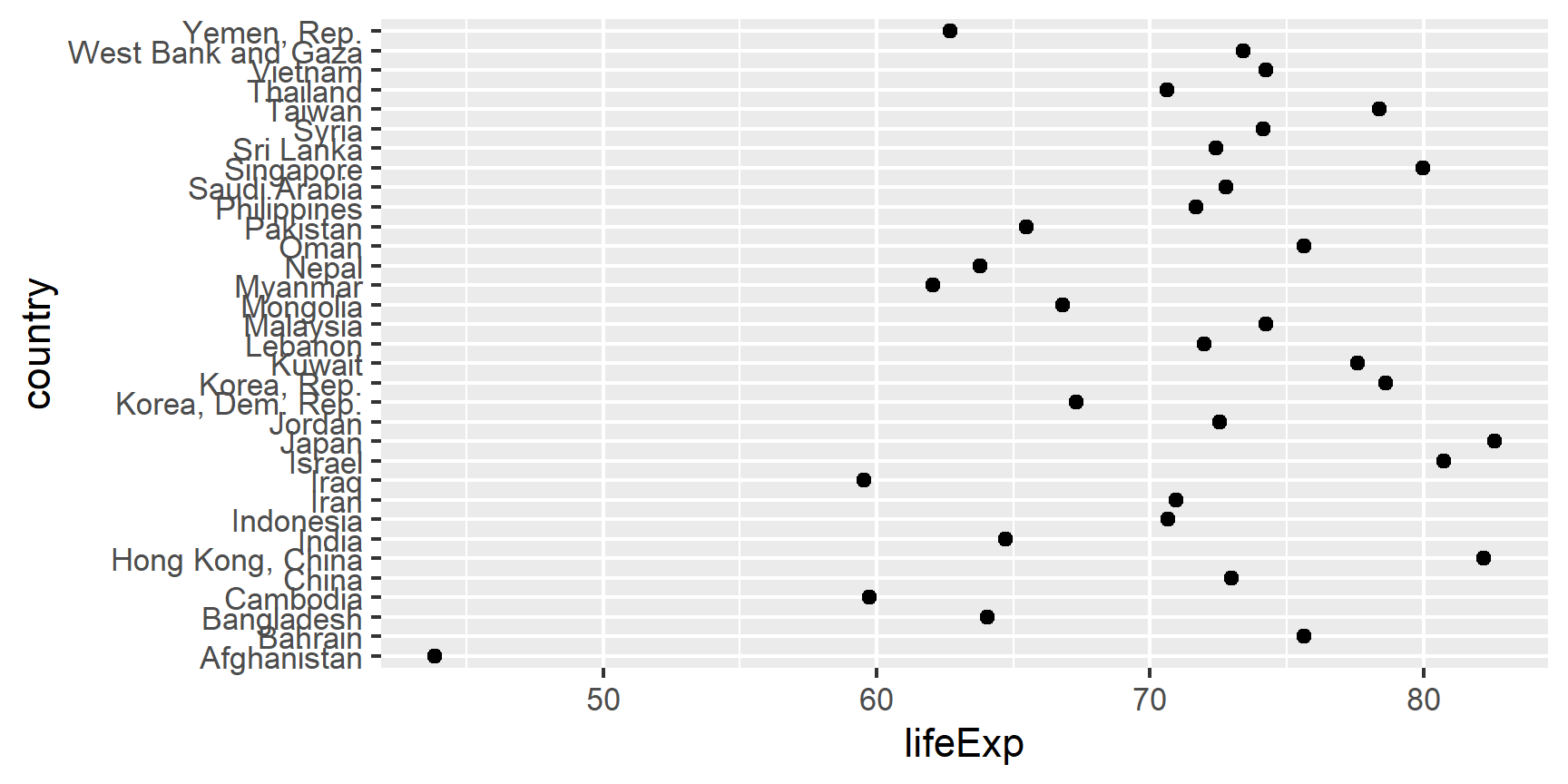
Example of why we reorder factor levels: often makes plots much better! When a factor is mapped to x or y, it should almost always be reordered by the quantitative variable you are mapping to the other one.
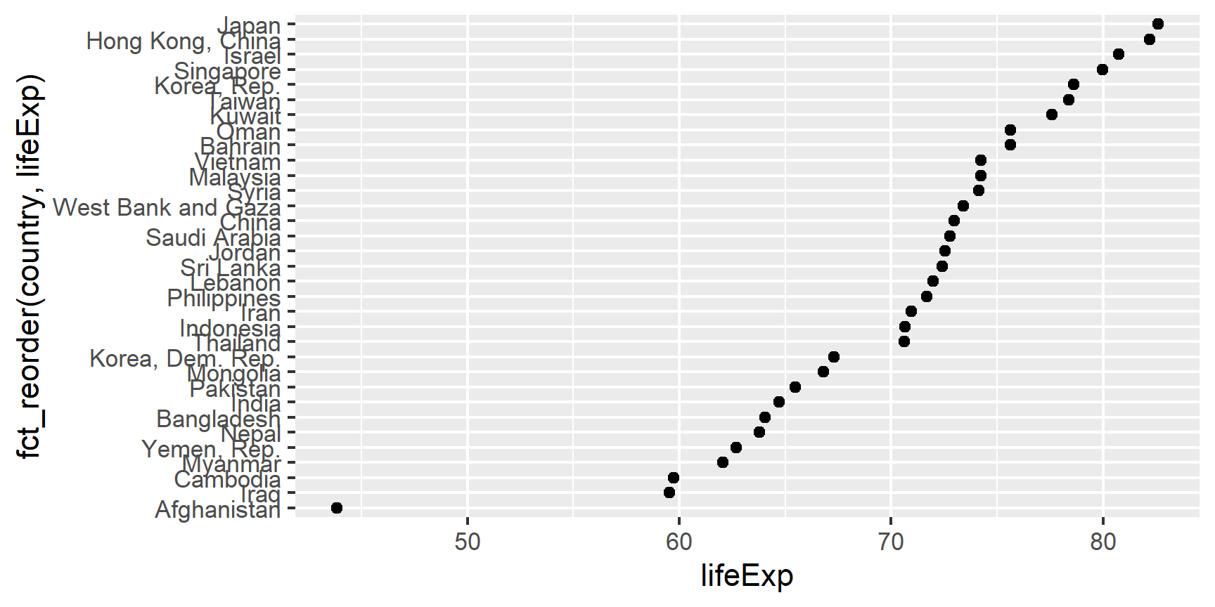
Compare the interpretability of these two plots of life expectancy in Asian
countries in 2007. The only difference is the order of the country factor.
Which one do you find easier to learn from?
gap_asia_2007 <- gapminder %>% filter(year == 2007, continent == "Asia")
ggplot(gap_asia_2007, aes(x = lifeExp, y = country)) + geom_point()
ggplot(gap_asia_2007, aes(x = lifeExp, y = fct_reorder(country, lifeExp))) +
  geom_point()
Use fct_reorder2() when you have a line chart of a quantitative x against
another quantitative y and your factor provides the color. This way the legend
appears in some order as the data! Contrast the legend on the left with the one
on the right.
renaming factor levels
forcats makes easy to rename factor levels. Let’s say we made a mistake and
need to recode “Oceania” to “Australia”. We’d use the fct_recode function to
do this.
levels(gapminder$continent)
## [1] "Africa" "Americas" "Asia" "Europe" "Oceania"
gapminder <- gapminder %>%
  mutate(continent_recode = fct_recode(continent, Australia = "Oceania"))

levels(gapminder$continent_recode)
## [1] "Africa" "Americas" "Asia" "Europe" "Australia"
There are many other forcat packages for very specific uses - like making an
“other” factor for rare occurrences with fct_lump(). Explore the cheatsheet so
you know what is available!
The lubridate Package

The lubridate package has many functions to simplify working with dates and times. The lubridate package does not come loaded as part of the tidyverse so you need to load it separately. Install the package if needed (using the console).
library(tidyverse)
library(lubridate)
Three main classes for date/time data

Datefor just the date.POSIXctfor both the date and the time (with Time Zone).- “POSIXct” stands for “Portable Operating System Interface - Calendar Time”. It is a part of a standardized system (based on UNIX) of representing time across many computing computing platforms.
hmsfrom thehmsR package for just the time. “hms” stands for “hours, minutes, and seconds.”
today() gives the current date in the Date class.
today()
## [1] "2021-03-27"
class(today())
## [1] "Date"
now() gives the current date-time in the POSIXct class.
now()
## [1] "2021-03-27 17:06:46 MST"
class(now())
## [1] "POSIXct" "POSIXt"
Parsing Dates and Times Using lubridate
lubridate has many "helper" functions which parse dates/times more automatically. - The helper *function name specifies the order of the components*: year, month, day, hours, minutes, and seconds. The help page forymd` shows multiple functions to parse dates with different sequences of
year, month and day,
Only the order of year, month, and day matters
ymd(c("2011/01-10", "2011-01/10", "20110110"))
## [1] "2011-01-10" "2011-01-10" "2011-01-10"
mdy(c("01/10/2011", "01 adsl; 10 df 2011", "January 10, 2011"))
## [1] "2011-01-10" "2011-01-10" "2011-01-10"
For times, only the order of hours, minutes, and seconds matter
hms(c("10:40:10", "10 40 10"))
## [1] "10H 40M 10S" "10H 40M 10S"
Let’s parse the following date-times.
t1 <- "05/26/2004 UTC 11:11:11.444"
t2 <- "26 2004 05 UTC 11/11/11.444"
mdy_hms(t1)
## [1] "2004-05-26 11:11:11 UTC"
## No dym_hms() function is defined, so need to use parse_datetime()
parse_date_time(t2, "d y m H M S")
## [1] "2004-05-26 11:11:11 UTC"
Now let’s use the appropriate lubridate function to parse the following dates:
d1 <- "January 1, 2010"
d2 <- "2015-Mar-07"
d3 <- "06-Jun-2017"
d4 <- c("August 19 (2015)", "July 1 (2015)")
d5 <- "12/30/14" # Dec 30, 2014
mdy(d1)
## [1] "2010-01-01"
ymd(d2)
## [1] "2015-03-07"
dmy(d3)
## [1] "2017-06-06"
mdy(d4)
## [1] "2015-08-19" "2015-07-01"
mdy(d5)
## [1] "2014-12-30"
Creating Date-time values from individual components
Use make_date() or make_datetime() to create dates and date-times if you
have a vector of years, months, days, hours, minutes, or seconds.
make_date(year = 1981, month = 6, day = 25)
## [1] "1981-06-25"
make_datetime(year = 1972, month = 2, day = 22, hour = 10, min = 9, sec = 01)
## [1] "1972-02-22 10:09:01 UTC"
You can see variables for the year, month, day, hour, and minute of the scheduled departure time with nycflights13 example:
library(nycflights13)
data("flights")

flights <- flights %>%
   mutate(datetime = make_datetime(year   = year,
                                  month  = month,
                                  day    = day,
                                  hour   = hour,
                                  min = minute))

select(flights, datetime)
## # A tibble: 336,776 x 1
##    datetime
##    <dttm>
##  1 2013-01-01 05:15:00
##  2 2013-01-01 05:29:00
##  3 2013-01-01 05:40:00
##  4 2013-01-01 05:45:00
##  5 2013-01-01 06:00:00
##  6 2013-01-01 05:58:00
##  7 2013-01-01 06:00:00
##  8 2013-01-01 06:00:00
##  9 2013-01-01 06:00:00
## 10 2013-01-01 06:00:00
## # ... with 336,766 more rows
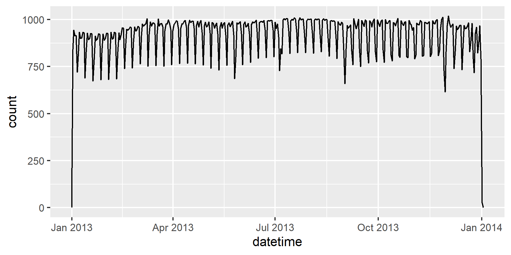
Having it in the date-time format makes it easier to plot.
ggplot(flights, aes(x = datetime)) +
  geom_freqpoly(bins = 365)
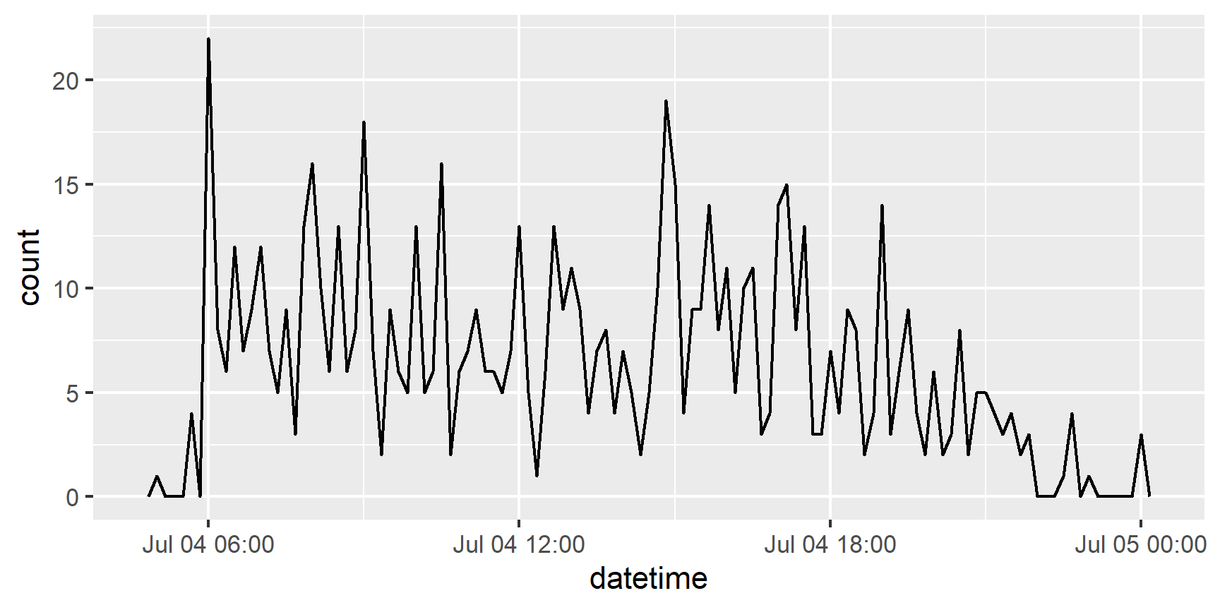
It also makes it easier to filter by date usingas_date() and ymd
flights %>%
  filter(as_date(datetime) == ymd(20130704)) %>%
  ggplot(aes(x = datetime)) +
  geom_freqpoly(binwidth = 600)
Extracting Components of a date-time
To extract the component of a date-time, use one of the following:
year()extracts the yearmonth()extracts the monthweek()extracts the weekmday()extracts the day of the month (1, 2, 3, …)wday()extracts the day of the week (Saturday, Sunday, Monday …)yday()extracts the day of the year (1, 2, 3, …)hour()extracts the hourminute()extract the minutesecond()extracts the second
ddat <- mdy_hms("01/02/1970 03:51:44")
ddat
## [1] "1970-01-02 03:51:44 UTC"
year(ddat)
## [1] 1970
month(ddat, label = TRUE)
## [1] Jan
## 12 Levels: Jan < Feb < Mar < Apr < May < Jun < Jul < Aug < Sep < ... < Dec
week(ddat)
## [1] 1
mday(ddat)
## [1] 2
wday(ddat, label = TRUE)
## [1] Fri
## Levels: Sun < Mon < Tue < Wed < Thu < Fri < Sat
yday(ddat)
## [1] 2
hour(ddat)
## [1] 3
minute(ddat)
## [1] 51
second(ddat)
## [1] 44
Doing Math with Time
Humans manipulate “clock time” with the use of policies such as Daylight
Savings Time which creates
irregularities in the “physical time”. lubridate provides three classes of
time spans to facilitate math with dates and date-times.
+ Periods: track changes in “clock time”, and ignore irregularities in
“physical time”.
+ Durations: track the passage of “physical time”, which deviates from
“clock time” when irregularities occur.
+ Intervals: represent specific spans of the timeline, bounded by start
and end date-times. We won’t cover this in this lesson, but you can learn
more with ?interval-class
Periods
Make a period with the name of a time unit pluralized, e.g.
p <- months(3) + days(12)
p
## [1] "3m 12d 0H 0M 0S"
str(p)
## Formal class 'Period' [package "lubridate"] with 6 slots
##   ..@ .Data : num 0
##   ..@ year  : num 0
##   ..@ month : num 3
##   ..@ day   : num 12
##   ..@ hour  : num 0
##   ..@ minute: num 0
You can read more about periods with
help("Period-class")
Durations
Durations are stored as seconds, the only time unit with a consistent length.
Add or subtract durations to model physical processes, like travel or
lifespan. You can create durations from years with dyears(), from days with
ddays(), etc…
dyears(1)
## [1] "31557600s (~1 years)"
ddays(1)
## [1] "86400s (~1 days)"
dhours(1)
## [1] "3600s (~1 hours)"
You can read about durations using
help("Duration-class")
You can also use duration(quantity, units = ...) to create a duration or
as.duration() to coerce an object to a duration. Example: We can find out the
exact age for the first single released by K-pop legends,
BTS using durations
d1 <- mdy("June 13, 2013")
d2 <- today()
str(d1)
## Date[1:1], format: "2013-06-13"
d2-d1
## Time difference of 2844 days
as.duration(d2 - d1)
## [1] "245721600s (~7.79 years)"