Tidy data and `tidyr`

Content for week of Monday, March 1, 2021–Thursday, March 4, 2021

Learning Outcomes

Describe tidy data
Make your data tidy with pivot_longer(), pivot_wider(), separate(), and unite().

Tidy Data

Data sets are often described in terms of three elements: units, variables and observations:
- Units: the items described by the data.
  - They may be Observational or Experimental.
  - They may be referred to as units, subjects, individuals, or cases or other terms.
  - They represent a population or a sample from a population, e.g., cars, people, or countries.
  - They are not the “units of measurement” but the items being measured.
  - They may be represented by variable, e.g., name, a combination of variables, e.g., country and year, or be implied and not explicitly represented by any variable (most common in summarized data), e.g., average scores for a group
- Variable: a characteristic or attribute of each unit about which we have data, e.g., mpg, age, or GDP.
- Observations: The single value for each variable for a given unit, e.g., 20 mpg, 31 years old, or $20,513,000 US.

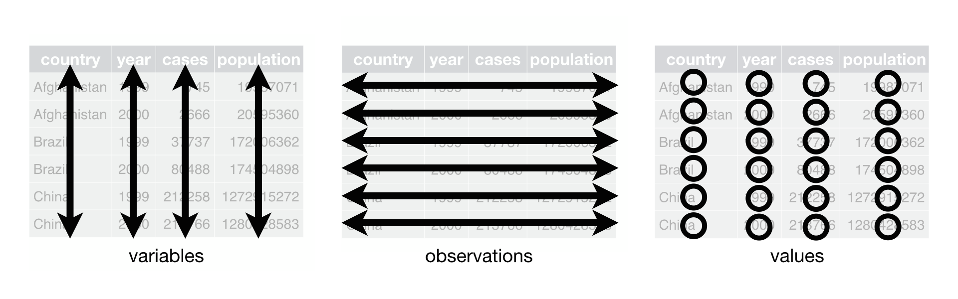
Definition of Tidy Data

We define tidy data very simply: It is a rectangular data set (the same number of rows for each column) where the data is shaped to have:

One unit per row.
One variable per column.
One observation (or value) per cell (the intersection of each row and column).

Hadley’s visualization:

The tidyr package is for Tidying or Reshaping Data

To tidy a data set, we change its “shape” so the variables and observations align to the columns and rows in accordance with our definition.
- Tidying is not about changing the attributes of the data such as variable type or the values of the observations or missing data.
- That is called cleaning the data
Today is about reshaping our data set to be in tidy format
We will use the tidyr package to make data tidy.
The tidyr package is part of the tidyverse. It is installed with it and also loaded and attached when you library(tidyverse)
Note, tidyr has two relatively new functions, pivot_longer() and pivot_wider(), which replace functions called gather() and spread() that are now deprecated. They still work and you will see them in web searches but they are not as capable as the new functions so we will focus on the new functions.
Let’s load the tidyverse

library(tidyverse)

A useful map of the tidyr functions

Examples of tidy and untidy data

Let’s look at multiple data sets on on wine consumption and population by country and year.
You will see there are many ways to be untidy.
We’ll start with a tidy version of the data
Tidy Data
- Units: Combinations of a Country and a Year - Note neither is an attribute of the other
- Variables: Country, Year, Cases Consumed, and Population
- One variable in each column and one observation for each unit in each row

table1

## # A tibble: 6 x 4
##   country      year  cases population
##   <chr>       <int>  <int>      <int>
## 1 Afghanistan  1999    745   19987071
## 2 Afghanistan  2000   2666   20595360
## 3 Brazil       1999  37737  172006362
## 4 Brazil       2000  80488  174504898
## 5 China        1999 212258 1272915272
## 6 China        2000 213766 1280428583

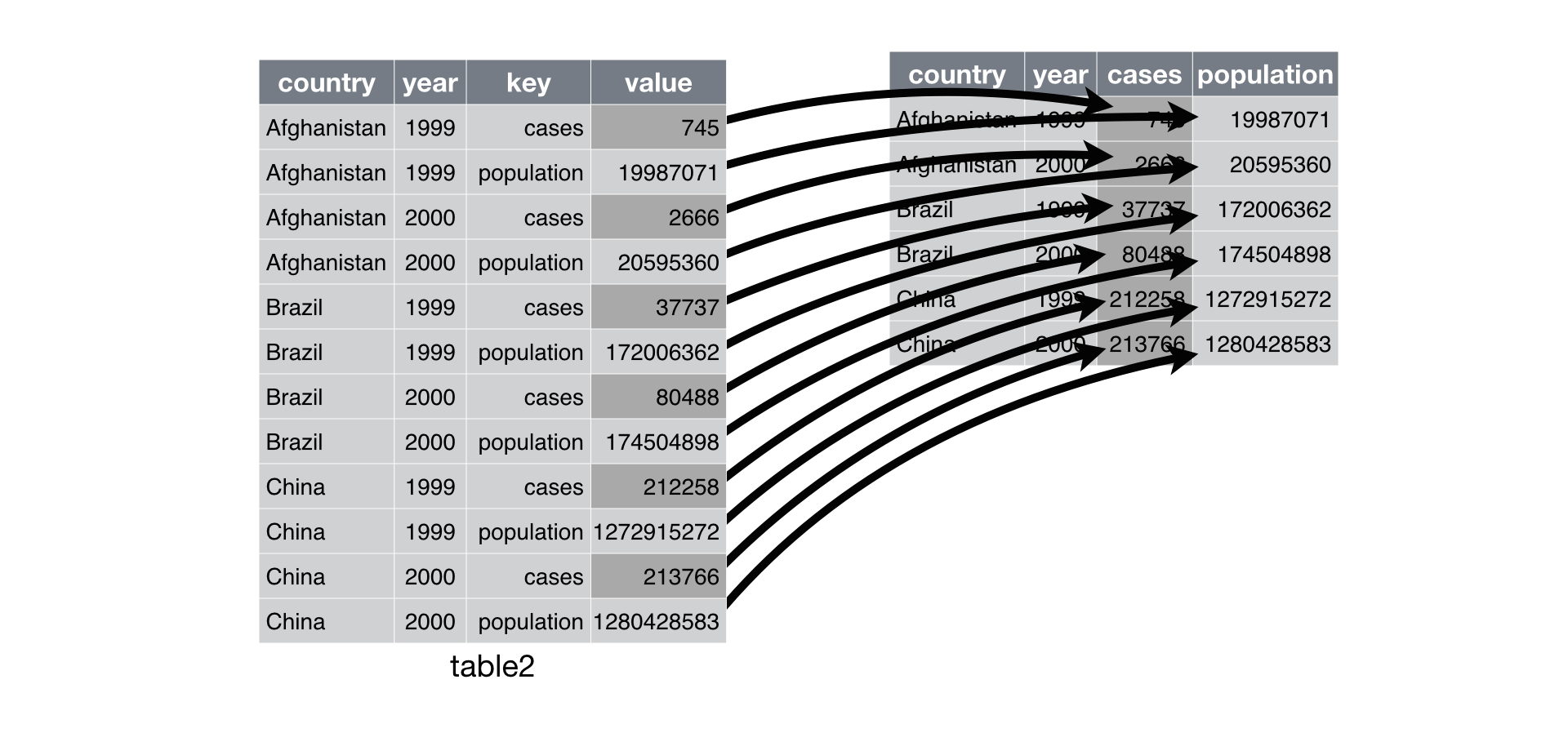
Untidy data where variables are combined in one column
- Same units and information but, …
- Two variables are in one column - type and their values are also in one column - count
- They are not different levels of the same variable

slice_head(table2, n = 12)

## # A tibble: 12 x 4
##    country      year type            count
##    <chr>       <int> <chr>           <int>
##  1 Afghanistan  1999 cases             745
##  2 Afghanistan  1999 population   19987071
##  3 Afghanistan  2000 cases            2666
##  4 Afghanistan  2000 population   20595360
##  5 Brazil       1999 cases           37737
##  6 Brazil       1999 population  172006362
##  7 Brazil       2000 cases           80488
##  8 Brazil       2000 population  174504898
##  9 China        1999 cases          212258
## 10 China        1999 population 1272915272
## 11 China        2000 cases          213766
## 12 China        2000 population 1280428583

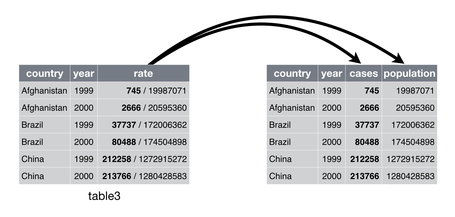
Untidy data where observations are combined into one column- rate

table3

## # A tibble: 6 x 3
##   country      year rate             
## * <chr>       <int> <chr>            
## 1 Afghanistan  1999 745/19987071     
## 2 Afghanistan  2000 2666/20595360    
## 3 Brazil       1999 37737/172006362  
## 4 Brazil       2000 80488/174504898  
## 5 China        1999 212258/1272915272
## 6 China        2000 213766/1280428583

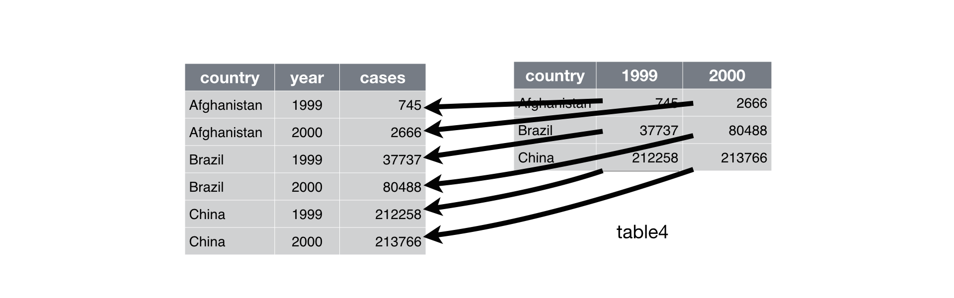
Untidy data where data of interest are spread across two data frames.
- Within each data frame, a variable is split into multiple columns.

table4a

## # A tibble: 3 x 3
##   country     `1999` `2000`
## * <chr>        <int>  <int>
## 1 Afghanistan    745   2666
## 2 Brazil       37737  80488
## 3 China       212258 213766

table4b

## # A tibble: 3 x 3
##   country         `1999`     `2000`
## * <chr>            <int>      <int>
## 1 Afghanistan   19987071   20595360
## 2 Brazil       172006362  174504898
## 3 China       1272915272 1280428583

Why Tidy Data

When data is tidy, it is shaped as individual vectors, usually columns in a data frame,
R and its tidyverse packages are designed to make it easy for you to manipulate vectors.
Sometimes it is easy to determine the units and the variables and the appropriate shape.
Sometimes it is hard.
- Talk with domain experts or the data collectors to find out the context with respect to the questions you are trying to answer.
- Can you distinguish the response variable(s) and potential explanatory variables?
In the long run, tidy data makes your life easier.
Let’s look at ways we can tidy our data.

Reshaping with `pivot_longer()`

(If you’re ever looking through older code, this used to be called gather.)

Problem: One Attribute (implied variable) Appears In Multiple Columns.

Column names are actually values of a implied variable
Examples in table4a and table4b

## # A tibble: 3 x 3
##   country     `1999` `2000`
##   <chr>        <int>  <int>
## 1 Afghanistan    745   2666
## 2 Brazil       37737  80488
## 3 China       212258 213766

## # A tibble: 3 x 3
##   country         `1999`     `2000`
##   <chr>            <int>      <int>
## 1 Afghanistan   19987071   20595360
## 2 Brazil       172006362  174504898
## 3 China       1272915272 1280428583

Solution: `pivot_longer()` to Convert Columns to Rows i.e., Make the Data Set Longer

Look at help for pivot_longer()
The first argument is the dataset to reshape (which you can pipe in)
The second argument cols = describes which columns need to be reshaped.
- You can use any of the tidyselect tidy helper functions, e.g., starts_with() or num_range()
- See “select” in help.
The names_to = is the name of the variable you want to create to hold the column names.
The values_to = is the name of the variable you want to create to hold the cell values.
Hadley’s visualization:

You have to specify three of the pivot_longer() arguments:
1. The columns that are values, not variables, with cols =
2. The name of the new variable with the old column names (names_to), and
3. The name of the new variable with the values spread across the current column cells (values_to).

table4a

## # A tibble: 3 x 3
##   country     `1999` `2000`
## * <chr>        <int>  <int>
## 1 Afghanistan    745   2666
## 2 Brazil       37737  80488
## 3 China       212258 213766

tidy4ap <- table4a %>%
  pivot_longer(cols = c(`1999`, `2000`), 
               names_to = "Year", 
               values_to = "Cases" ) 
tidy4ap

## # A tibble: 6 x 3
##   country     Year   Cases
##   <chr>       <chr>  <int>
## 1 Afghanistan 1999     745
## 2 Afghanistan 2000    2666
## 3 Brazil      1999   37737
## 4 Brazil      2000   80488
## 5 China       1999  212258
## 6 China       2000  213766

table4b

## # A tibble: 3 x 3
##   country         `1999`     `2000`
## * <chr>            <int>      <int>
## 1 Afghanistan   19987071   20595360
## 2 Brazil       172006362  174504898
## 3 China       1272915272 1280428583

tidy4bp <- table4b %>%
  pivot_longer(cols = c('1999', '2000'), 
               names_to = "Year", 
               values_to = "Population") 
tidy4bp

## # A tibble: 6 x 3
##   country     Year  Population
##   <chr>       <chr>      <int>
## 1 Afghanistan 1999    19987071
## 2 Afghanistan 2000    20595360
## 3 Brazil      1999   172006362
## 4 Brazil      2000   174504898
## 5 China       1999  1272915272
## 6 China       2000  1280428583

We will learn next class how to join two data frames but for now we will use dplyr:: left_join()

tidy4ap %>% 
  left_join(tidy4bp, by = c("country","Year"))

## # A tibble: 6 x 4
##   country     Year   Cases Population
##   <chr>       <chr>  <int>      <int>
## 1 Afghanistan 1999     745   19987071
## 2 Afghanistan 2000    2666   20595360
## 3 Brazil      1999   37737  172006362
## 4 Brazil      2000   80488  174504898
## 5 China       1999  212258 1272915272
## 6 China       2000  213766 1280428583

Exercises

Tidy the monkeymem data frame (available at https://dcgerard.github.io/stat_412_612/data/monkeymem.csv). The cell values represent identification accuracy of some objects (in percent of 20 trials).

monkeymem <- read_csv("https://dcgerard.github.io/stat_412_612/data/monkeymem.csv")
glimpse(monkeymem)

monkeymem %>%
  pivot_longer( )

Why does this code fail?

table4a %>% 
  pivot_longer(cols = 1999, 2000, 
               names_to = "year", 
               values_to = "cases")

1999 and 2000 are prohibited variable names. You can get around this by surrounding them with single quotes and combining into a character vector as in our prior example.

Reshaping with `pivot_wider()`

(If you’re ever looking through older code, this used to be called spread())

Problem: One Observation’s Attributes Appear in Multiple rows.

One column contains variable names.
One column contains values for the different attributes i.e., implied variables.
This can be more challenging to tidy as you have multiple variables to address
Example is table2

## # A tibble: 6 x 4
##   country      year type           count
##   <chr>       <int> <chr>          <int>
## 1 Afghanistan  1999 cases            745
## 2 Afghanistan  1999 population  19987071
## 3 Afghanistan  2000 cases           2666
## 4 Afghanistan  2000 population  20595360
## 5 Brazil       1999 cases          37737
## 6 Brazil       1999 population 172006362

Solution: `pivot_wider()` to Convert Rows to Columns, i.e., Make the Data Set Wider

See help for pivot_wider()
The first argument is the data frame to pivot.
id_cols= specifies the set of columns which together uniquely identify each observation.
- Usually the default is okay.
- It uses all the other columns in the data except for the columns in names_from and values_from.
names_from = says which column (or columns) to use to get the new variable name of the output columns.
values_from = says which column (or columns) to use to get the cell values from for the new variables.
Hadley’s visualization:

Specify at least two arguments in addition to the data frame:
1. The column with the column names (names_from =), and
2. The column with the values (values_from = ).

table2

## # A tibble: 12 x 4
##    country      year type            count
##    <chr>       <int> <chr>           <int>
##  1 Afghanistan  1999 cases             745
##  2 Afghanistan  1999 population   19987071
##  3 Afghanistan  2000 cases            2666
##  4 Afghanistan  2000 population   20595360
##  5 Brazil       1999 cases           37737
##  6 Brazil       1999 population  172006362
##  7 Brazil       2000 cases           80488
##  8 Brazil       2000 population  174504898
##  9 China        1999 cases          212258
## 10 China        1999 population 1272915272
## 11 China        2000 cases          213766
## 12 China        2000 population 1280428583

table2 %>%
  pivot_wider(id_cols = c(country, year),
              names_from = type, 
              values_from = count)

## # A tibble: 6 x 4
##   country      year  cases population
##   <chr>       <int>  <int>      <int>
## 1 Afghanistan  1999    745   19987071
## 2 Afghanistan  2000   2666   20595360
## 3 Brazil       1999  37737  172006362
## 4 Brazil       2000  80488  174504898
## 5 China        1999 212258 1272915272
## 6 China        2000 213766 1280428583

Exercises:

Tidy (reshape) the flowers1 data frame (available at https://dcgerard.github.io/stat_412_612/data/flowers1.csv).

flowers1 <- read_csv2("https://dcgerard.github.io/stat_412_612/data/flowers1.csv")
slice(flowers1,20:28)

flowers1 %>% 
  pivot_wider()

## # A tibble: 9 x 4
##    Time replication Variable  Value
##   <dbl>       <dbl> <chr>     <dbl>
## 1     2           8 Flowers    52.2
## 2     2           9 Flowers    60.3
## 3     2          10 Flowers    45.6
## 4     2          11 Flowers    52.6
## 5     2          12 Flowers    44.4
## 6     1           1 Intensity 150  
## 7     1           2 Intensity 150  
## 8     1           3 Intensity 300  
## 9     1           4 Intensity 300

## # A tibble: 24 x 4
##     Time replication Flowers Intensity
##    <dbl>       <dbl>   <dbl>     <dbl>
##  1     1           1    62.3       150
##  2     1           2    77.4       150
##  3     1           3    55.3       300
##  4     1           4    54.2       300
##  5     1           5    49.6       450
##  6     1           6    61.9       450
##  7     1           7    39.4       600
##  8     1           8    45.7       600
##  9     1           9    31.3       750
## 10     1          10    44.9       750
## # ... with 14 more rows

(RDS 13.3.3.3): Why does using pivot_wider on this data frame fail?

people <- tribble(
  ~name,             ~key,    ~value,
  #-----------------|--------|------
  "Phillip Woods",   "age",       45,
  "Phillip Woods",   "height",   186,
  "Phillip Woods",   "age",       50,
  "Jessica Cordero", "age",       37,
  "Jessica Cordero", "height",   156
)

There is a duplicate row for “Phillip Woods” and “Age”. So in the “Phillip Woods” row and “age” column, should we put in 45 or 50?
pivot_wider() doesn’t know what to do so it throws an error.

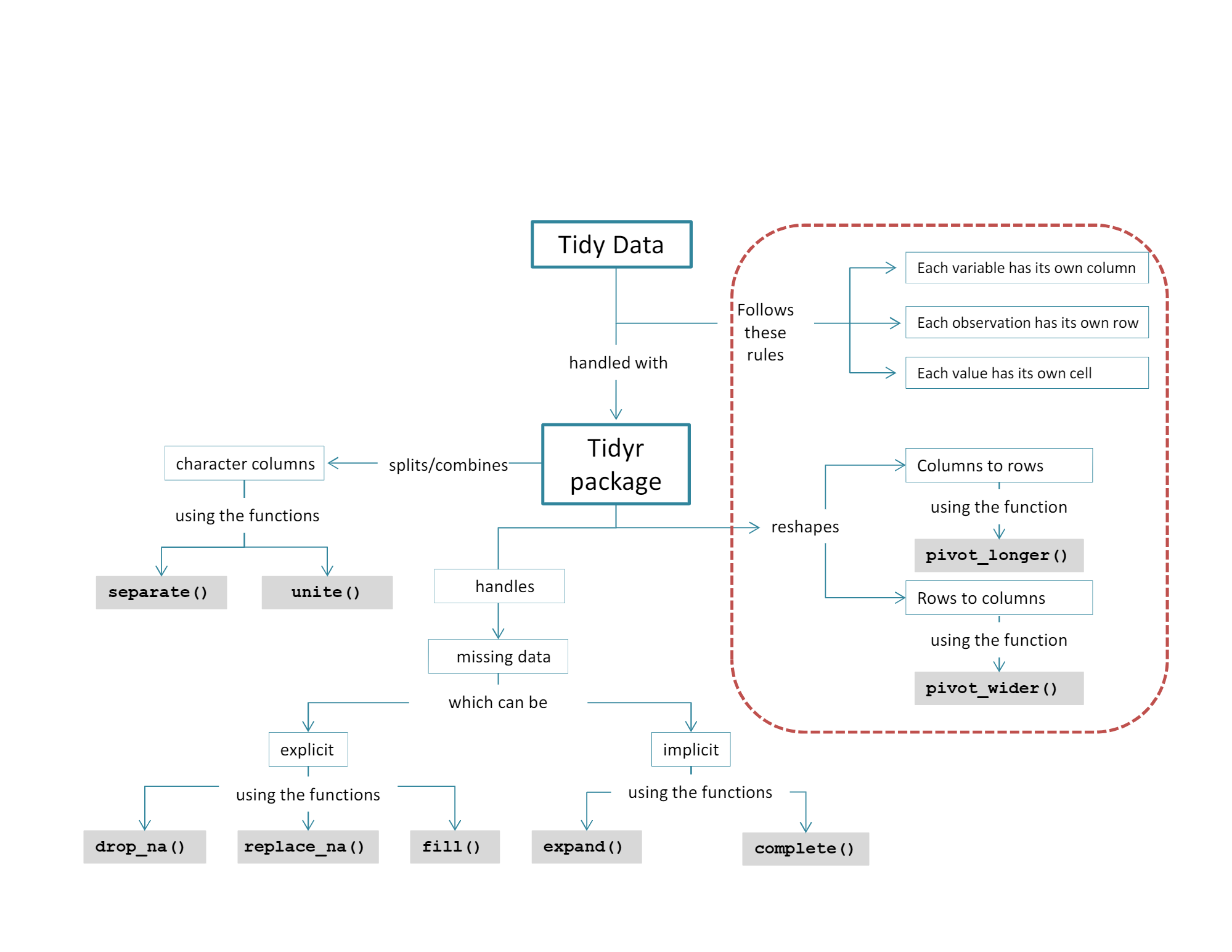
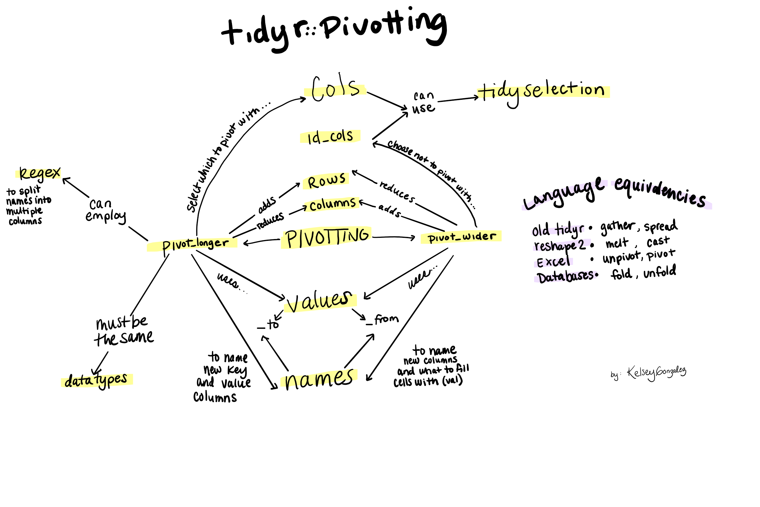
If you get lost between pivot_wider() and pivot_longer(), I suggest drawing yourself a concept map like the one below, which I drew for myself.

pivotting concept map

`separate()` Combined Data Values

Problem: One Column Contains Values from Two (or more) Variables in Each Row.

Example is table3

## # A tibble: 6 x 3
##   country      year rate             
##   <chr>       <int> <chr>            
## 1 Afghanistan  1999 745/19987071     
## 2 Afghanistan  2000 2666/20595360    
## 3 Brazil       1999 37737/172006362  
## 4 Brazil       2000 80488/174504898  
## 5 China        1999 212258/1272915272
## 6 China        2000 213766/1280428583

Solution: `separate()`

See help for separate()
First argument is the data frame (from %>% usually)
col = the name or position of the column to be separated
into = a character vector of the names of the new variables.
- You can use NA to drop one that is not of interest
sep = The separator you want to use to split the data into new columns
- If a character, e.g. “-” seen as a REGEX (beware of backslashes, periods, …).
- If a numeric, the positions where to split the data
  - If positive, counting from left to right
  - If negative, counting from right to left
  - Should have length(sep) = length (into) -1
Hadley’s visualization:

You need to specify at least three arguments:
1. The column you want to separate that has two (or more) variables,
2. The character vector of the names of the new variables, and
3. The character or numeric positions by which to separate out the new variables from the current column.

head(table3)

## # A tibble: 6 x 3
##   country      year rate             
##   <chr>       <int> <chr>            
## 1 Afghanistan  1999 745/19987071     
## 2 Afghanistan  2000 2666/20595360    
## 3 Brazil       1999 37737/172006362  
## 4 Brazil       2000 80488/174504898  
## 5 China        1999 212258/1272915272
## 6 China        2000 213766/1280428583

table3 %>%
  separate(rate, 
           into = c("cases", "population"), 
           sep = "/")

## # A tibble: 6 x 4
##   country      year cases  population
##   <chr>       <int> <chr>  <chr>     
## 1 Afghanistan  1999 745    19987071  
## 2 Afghanistan  2000 2666   20595360  
## 3 Brazil       1999 37737  172006362 
## 4 Brazil       2000 80488  174504898 
## 5 China        1999 212258 1272915272
## 6 China        2000 213766 1280428583

Exercise

Tidy the flowers2 data frame (available at https://dcgerard.github.io/stat_412_612/data/flowers2.csv).

flowers2 <- read_csv2("https://dcgerard.github.io/stat_412_612/data/flowers2.csv")
head(flowers2)

flowers2_sep <- flowers2 %>%
  separate()

## # A tibble: 6 x 2
##   `Flowers/Intensity`  Time
##   <chr>               <dbl>
## 1 62.3/150                1
## 2 77.4/150                1
## 3 55.3/300                1
## 4 54.2/300                1
## 5 49.6/450                1
## 6 61.9/450                1

`unite()` Values from Multiple Columns to Create a New Variable

Problem: One Variable Spread Across Multiple Columns.

This is a much less common problem.
You can see it with dates and/or times
Example has Year split into century and two-digit year

## # A tibble: 6 x 4
##   country     century year  rate             
##   <chr>       <chr>   <chr> <chr>            
## 1 Afghanistan 19      99    745/19987071     
## 2 Afghanistan 20      00    2666/20595360    
## 3 Brazil      19      99    37737/172006362  
## 4 Brazil      20      00    80488/174504898  
## 5 China       19      99    212258/1272915272
## 6 China       20      00    213766/1280428583

Solution: `unite()` Multiple Columns to Create a New Variable

See help for unite()
Note you can either remove (the default) or keep the original columns
Hadley’s visualization:

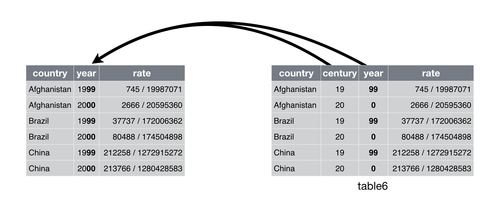
You must specify three arguments:
1. The name of the new column (col),
2. The columns to unite, and
3. The separator of the variables in the new column (sep) if none use ("")

table5 %>%
  unite( col = "Year",  # new name
         century, year,  #unite these cols
         sep = "" #if you want a delimiter
         )

## # A tibble: 6 x 3
##   country     Year  rate             
##   <chr>       <chr> <chr>            
## 1 Afghanistan 1999  745/19987071     
## 2 Afghanistan 2000  2666/20595360    
## 3 Brazil      1999  37737/172006362  
## 4 Brazil      2000  80488/174504898  
## 5 China       1999  212258/1272915272
## 6 China       2000  213766/1280428583

Exercises

Re-unite the data frame you separated from the flowers2 exercise.

Use a comma for the separator.

flowers2_sep %>%
  unite()

## # A tibble: 24 x 2
##    `Flowers,Intensity`  Time
##    <chr>               <dbl>
##  1 62.3,150                1
##  2 77.4,150                1
##  3 55.3,300                1
##  4 54.2,300                1
##  5 49.6,450                1
##  6 61.9,450                1
##  7 39.4,600                1
##  8 45.7,600                1
##  9 31.3,750                1
## 10 44.9,750                1
## # ... with 14 more rows

Use the flights data from the nycflights13 package.

Select the month, day, hour and minute.
Combine the hour and minute into a new variable sd_time and convert into a time object
What happened and why?
We can fix using the stringr package (a few weeks from now)
References
- Chapter 12 of RDS
- Data Import Cheat Sheet
- Tidyr Overview.
- Pivot Vignette
- TidyR Slides by Palolili23

Last updated on March 1, 2021

Edit this page

Tidy data and `tidyr`

Learning Outcomes

Tidy Data

Definition of Tidy Data

The tidyr package is for Tidying or Reshaping Data

Examples of tidy and untidy data

Why Tidy Data

Reshaping with pivot_longer()

Problem: One Attribute (implied variable) Appears In Multiple Columns.

Solution: pivot_longer() to Convert Columns to Rows i.e., Make the Data Set Longer

Exercises

Reshaping with pivot_wider()

Problem: One Observation’s Attributes Appear in Multiple rows.

Solution: pivot_wider() to Convert Rows to Columns, i.e., Make the Data Set Wider

Exercises:

separate() Combined Data Values

Problem: One Column Contains Values from Two (or more) Variables in Each Row.

Solution: separate()

Exercise

unite() Values from Multiple Columns to Create a New Variable

Problem: One Variable Spread Across Multiple Columns.

Solution: unite() Multiple Columns to Create a New Variable

Exercises

Reshaping with `pivot_longer()`

Solution: `pivot_longer()` to Convert Columns to Rows i.e., Make the Data Set Longer

Reshaping with `pivot_wider()`

Solution: `pivot_wider()` to Convert Rows to Columns, i.e., Make the Data Set Wider

`separate()` Combined Data Values

Solution: `separate()`

`unite()` Values from Multiple Columns to Create a New Variable

Solution: `unite()` Multiple Columns to Create a New Variable