Lab 1
You’ll be doing all your R work in R Markdown this time (and from now on). You should use an RStudio Project to keep your files well organized. Either create a new project for this exercise only, or make a project for all your work in this class.
Task 1: Make an RStudio Project
-
Use RStudio on your computer Follow these instructions if you never got it downloaded to create a new RStudio Project named “STAT412-612” if you didn’t make one during our class.
-
Create a folder named “data” in the project folder. Create the following folders as well: “lecture-notes”, “labs”, “homework”, “output”.
-
Download this CSV file and place it in your data folder:
-
In RStudio, go to “File” > “New File…” > “R Markdown…” and click “OK” in the dialog without changing anything.
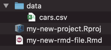
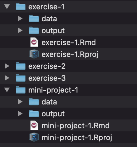
Your structure should look something like this:
Task 2: Work with R Markdown
I suggest you knit after each of these steps to make sure it looks right!
-
In the YAML heading (the text between
---), Write a title, your name, and that you want to output to html -
After the closing YAML (after the second
---), delete all the auto-generated text and create a level-1 header. Under that new header, introduce yourself. Tell me your name, major, favorite late night snack. Be sure to use italics, bold, and othertricks. -
Add the following questions as level 2 headers and write a sentence responding to each.
- What do you need from me to be successful this semester?
- What is something non-academic related you’re passionate about?
- What’s something you did or learned in 2020 to stay sane?
-
Add a picture of your favorite animal.
-
Save the R Markdown file in your “lab” folder with some sort of name that indicates this is for lab 1 (without any spaces!)
Task 3: Work with R
-
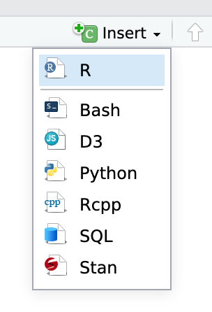
Add a new level 1 header named “R code” and create an R code chunk underneath. Either type ctrl + alt + i on Windows, or ⌘ + ⌥ + i on macOS, or use the “Insert Chunk” menu:
-
In the code chunk, load the
treesdataset. -
Practice using some of the data exploration commands that were introduced in class. How many can you remember and use?
-
Load the cars.csv dataset you downloaded using
cars <- read.csv("data/cars.csv"). We’ll go over this syntax in more detail in week 4. What are some differences between the two datasets (trees and cars), particularly in the types of data stored in the columns? -
Check your spelling using Edit -> Check/Spelling of the
ABC🗸next to the save icon. -
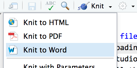
Knit your document as an HTML file (or PDF if you’re brave and installed LaTeX). Use the “Knit” menu:
-
Upload the knitted document and the
.Rmdfiles to Canvas. -
🎉 Party! 🎉
If you’re done early, I want to install the tidyverse. Run install.packages("tidyverse") Some more detailed steps are in your textbook at 1.4.3. This will usually take about 3 minutes and I don’t want to use class time to do so. To verify it installed correctly, run library(tidyverse) without receiving any errors.
You’ll be doing this same process for all your future labs. Each problem set will involve an R Markdown file. You can either create a new RStudio Project directory for all your work:
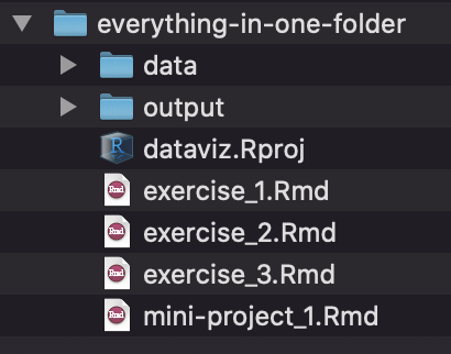
Or you can create individual projects for each assignment and project:
On Canvas, you will turn in your .Rmd, .html, and/or .pdf file.